Appearance Features

Audiovisual Processing CMP-6026A

Dr. David Greenwood

Content

DCT Features
Eigenfaces
Appearance Models
Visual Feature Efficacy
Model Fusion

Image-based Features

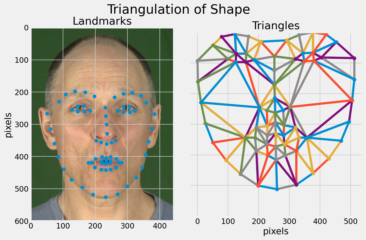
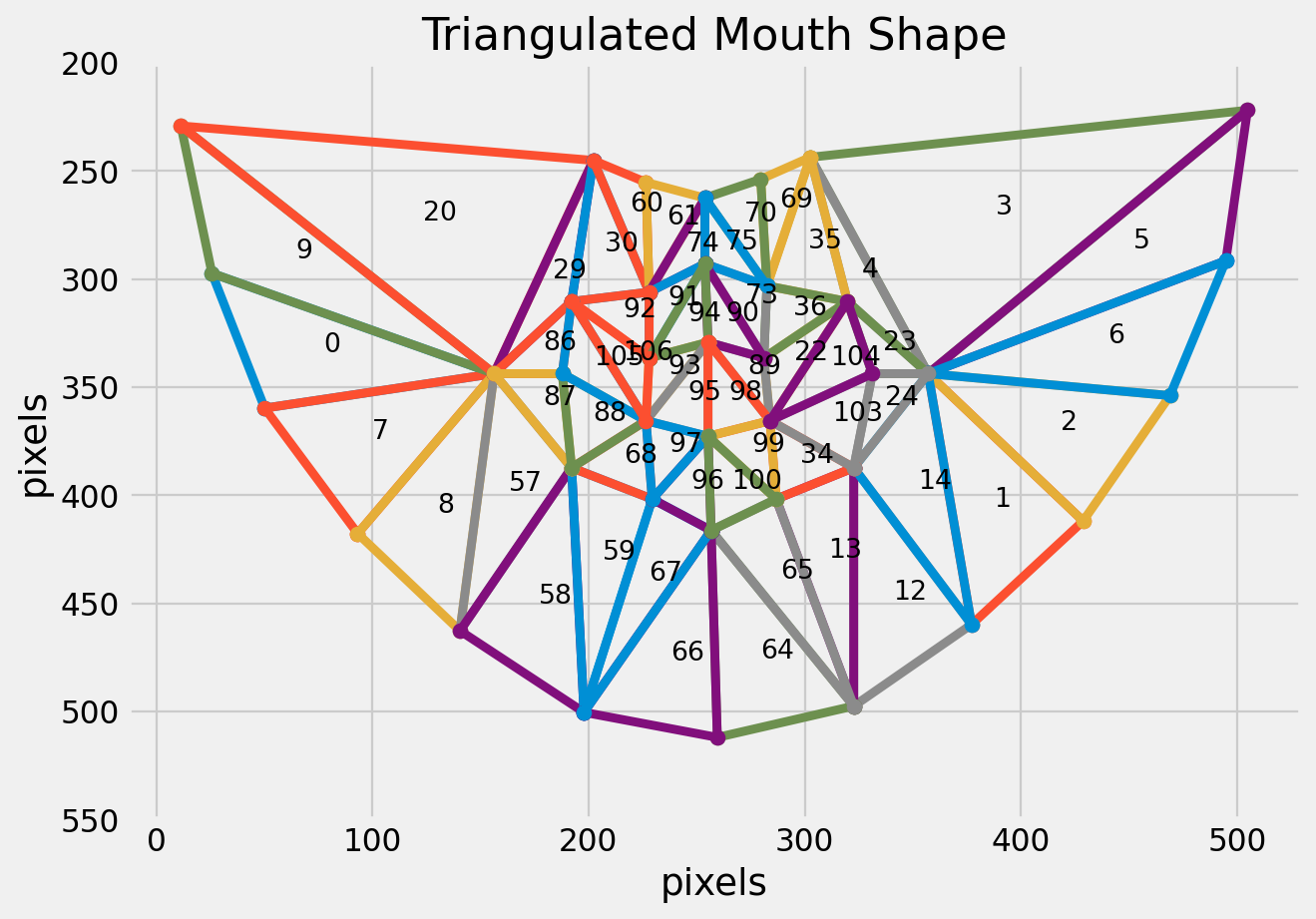
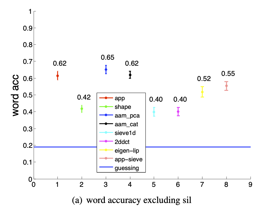
The main limitation of shape-only features is there is a lot of information missing.

Modelling only lip-shape discards information about the teeth and tongue for example.
Why not use the full appearance of the face?

DCT Features

Discrete Cosine Transform (DCT)

Performs a similar function to DFT in that it transforms a signal (or image) from the spatial domain to the frequency domain.

The difference is that it only considers the real-valued cosine components of the DFT.
We can compact the energy of the signal into the low frequency bins.
Used in JPEG compression.
First proposed by Nasir Ahmed in 1972.

Review: DFT

DCT 1D

\[ X_k = s(k) ~ \sum_{n=0}^{N-1} x_n cos \left[ \frac{\pi k (2n + 1)}{2N} \right] \]

Where:

\(X\) is the DCT output
\(x\) is the input signal
\(N\) is the number of samples
\(k = 0, 1, 2, \dots, N-1\)
\(s(0) = \sqrt{1/N}, ~ s(k \neq 0) = \sqrt{2/N}\)

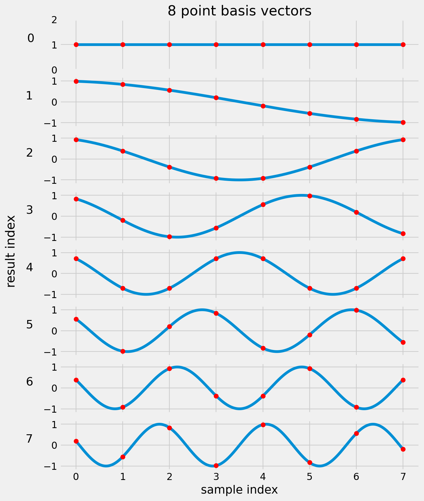
8-Point 1-D DCT Basis

\[Y_k = cos \left[ \frac{\pi k (2n + 1)}{2N} \right]\]

\[n = 0, 1, 2, \dots, N-1\]

DCT for 1D Signals

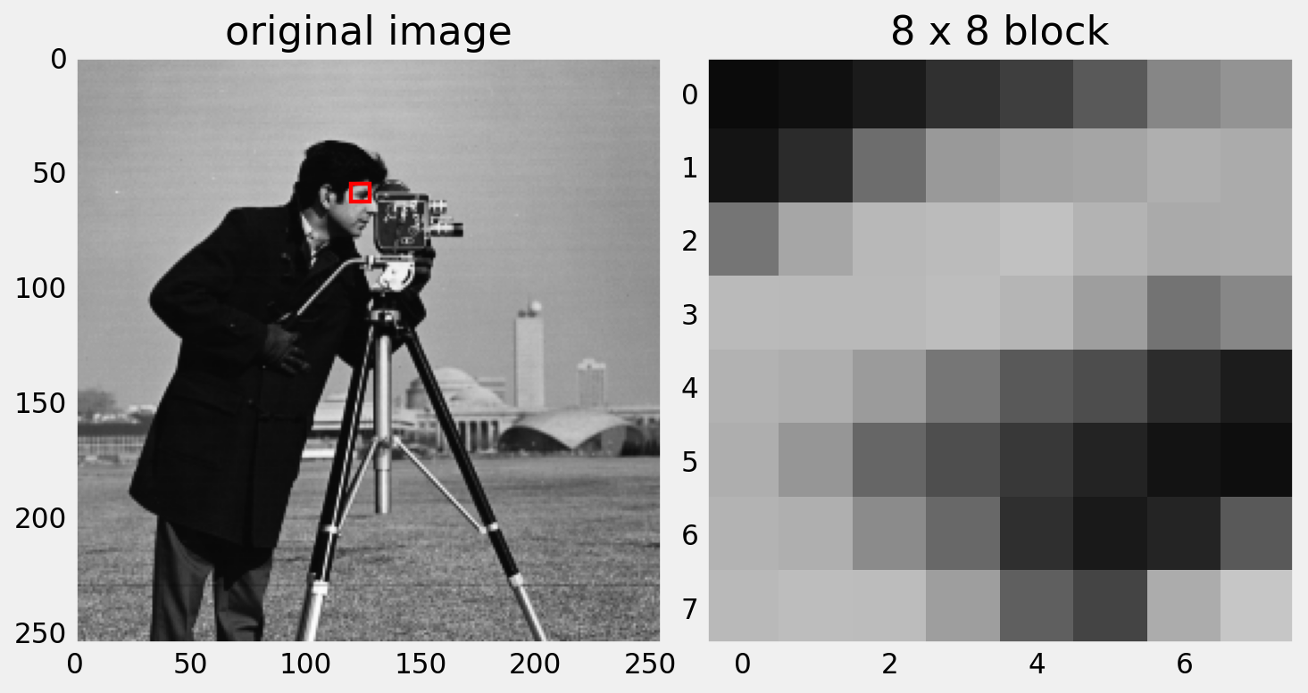
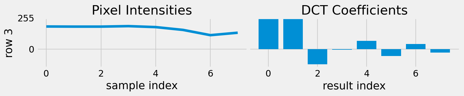
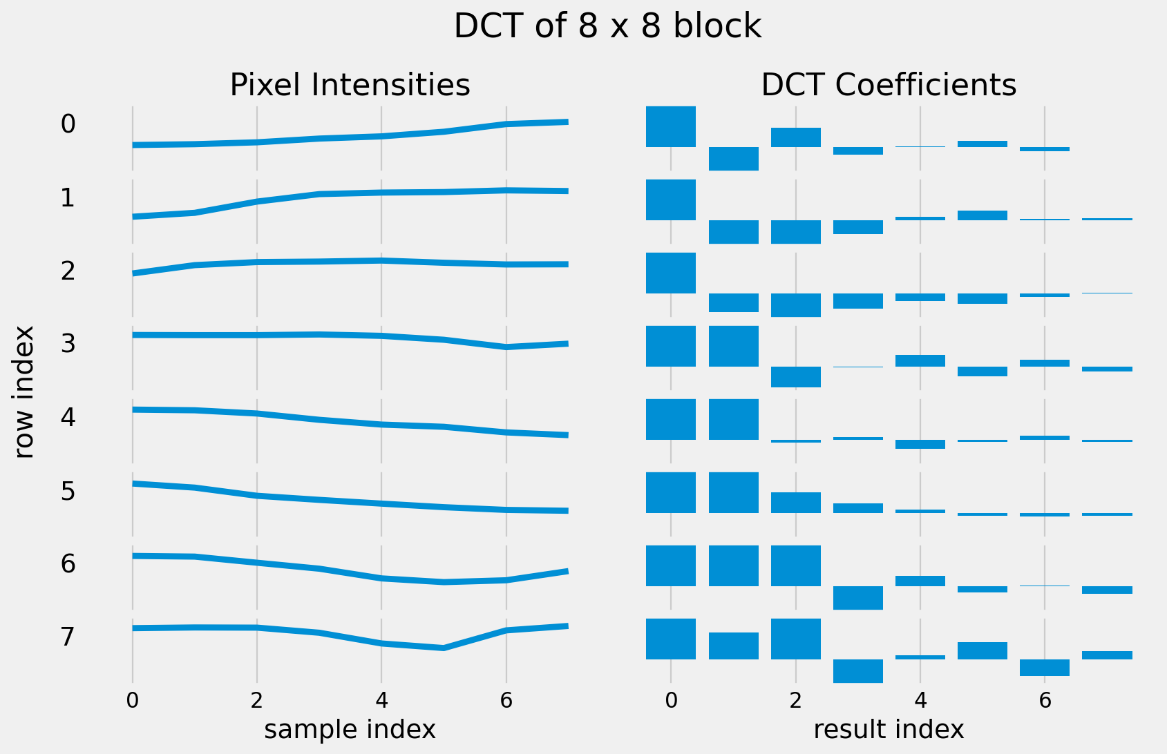
Let’s look at one 8 x 8 block in an image.

DCT for 1D Signals

Most of the energy is concentrated in the low frequency coefficients.
Images have less high frequency information.

DCT for 2D Signals

We have only considered vectors so far.

Images are 2-dimensional (two spatial co-ordinates).
Apply DCT to both rows and columns of the image.

\[ X_{u, v} = s_u s_v ~ \sum_{x=0}^{N-1} \sum_{y=0}^{N-1} I(x, y) ~ cos \left[ \frac{\pi u (2x + 1)}{2N} \right] cos \left[ \frac{\pi v (2y + 1)}{2N} \right] \]

DCT for 2D Signals

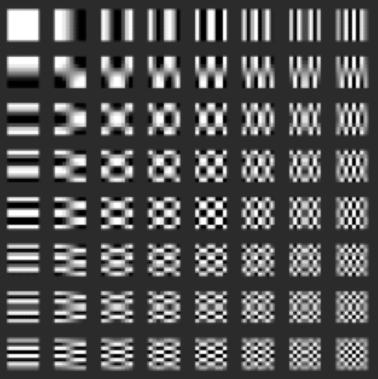
Rather than basis vectors, we have basis images.

DCT for 2D Signals

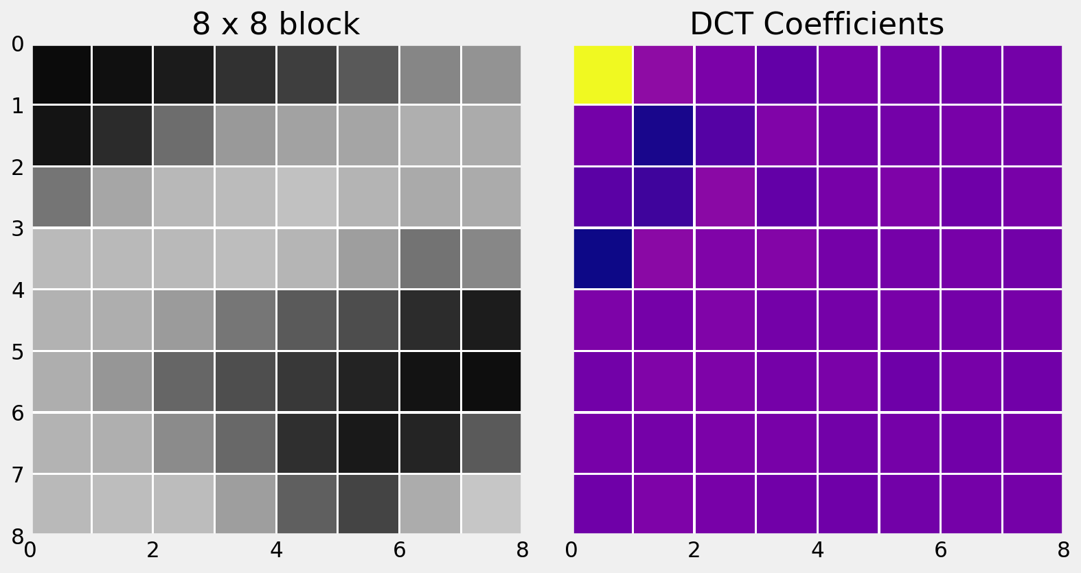
Let’s look again at the same 8 x 8 block in an image.

DCT for 2D Signals

Here is the 2D DCT of the block.

DCT for 2D Signals

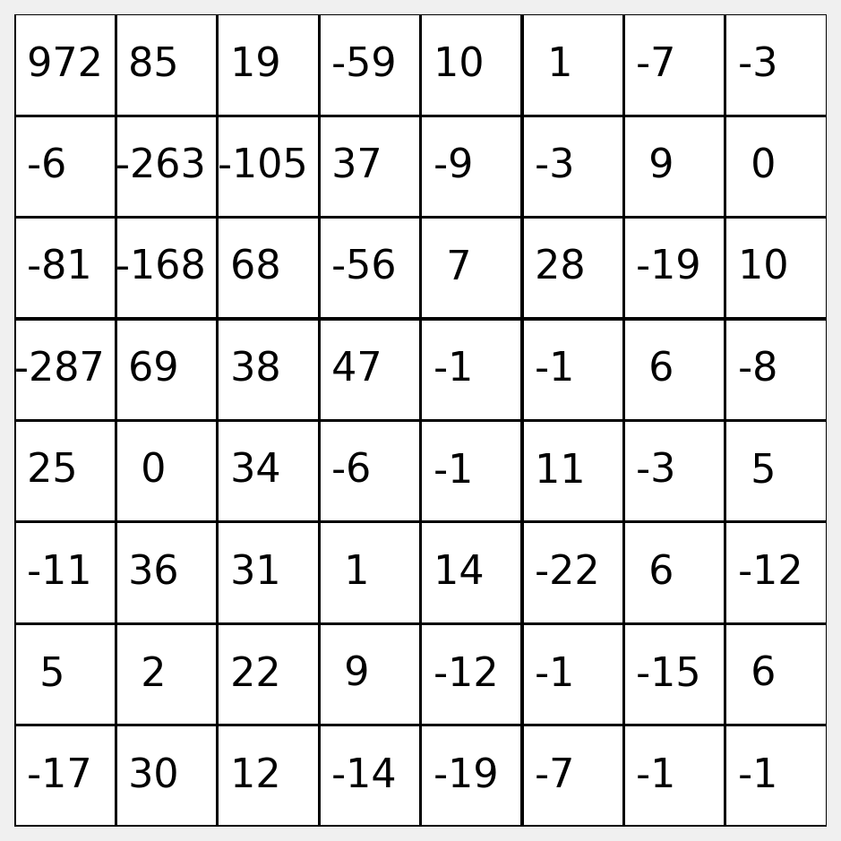
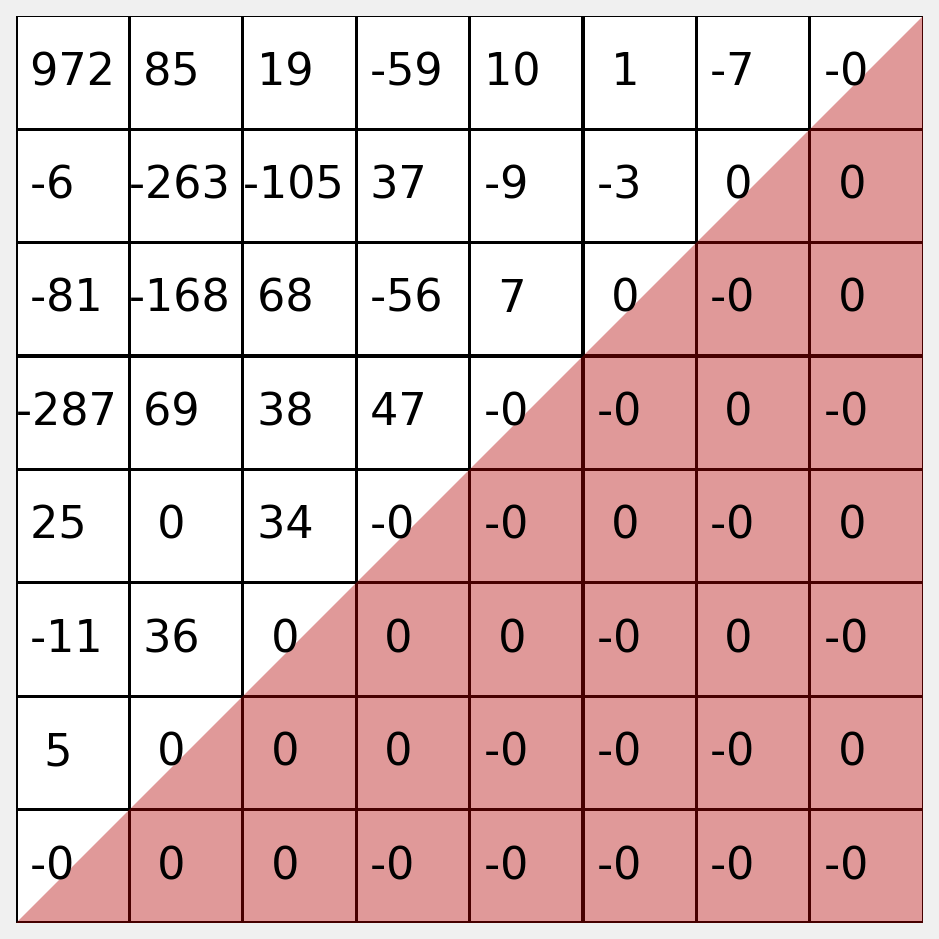
Let’s examine the actual values of the coefficients.

DCT for 2D Signals

Notice that the most significant values congregate at the top left.

DCT for 2D Signals

We can stack the top left values to make a feature vector.

\(f = (972, 85, 19, -59, \dots)\)

DCT for 2D Signals

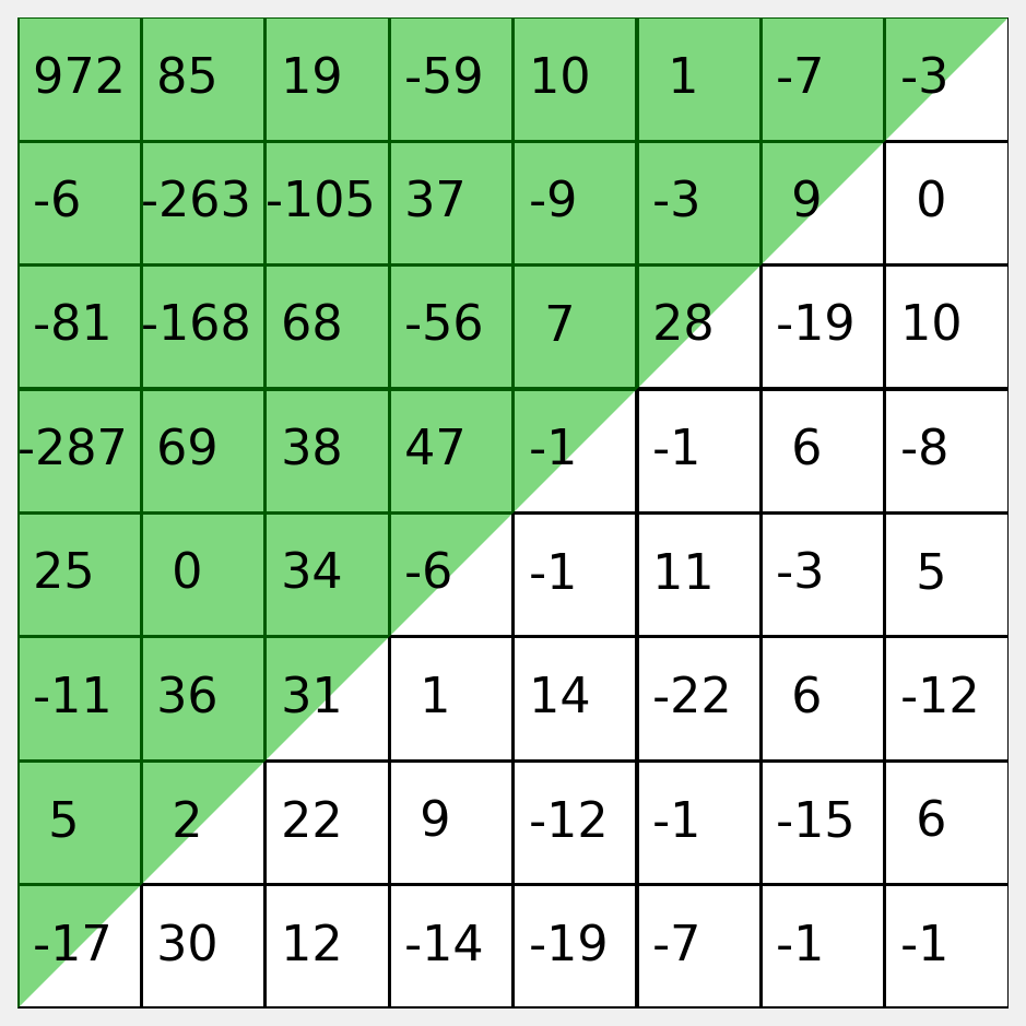
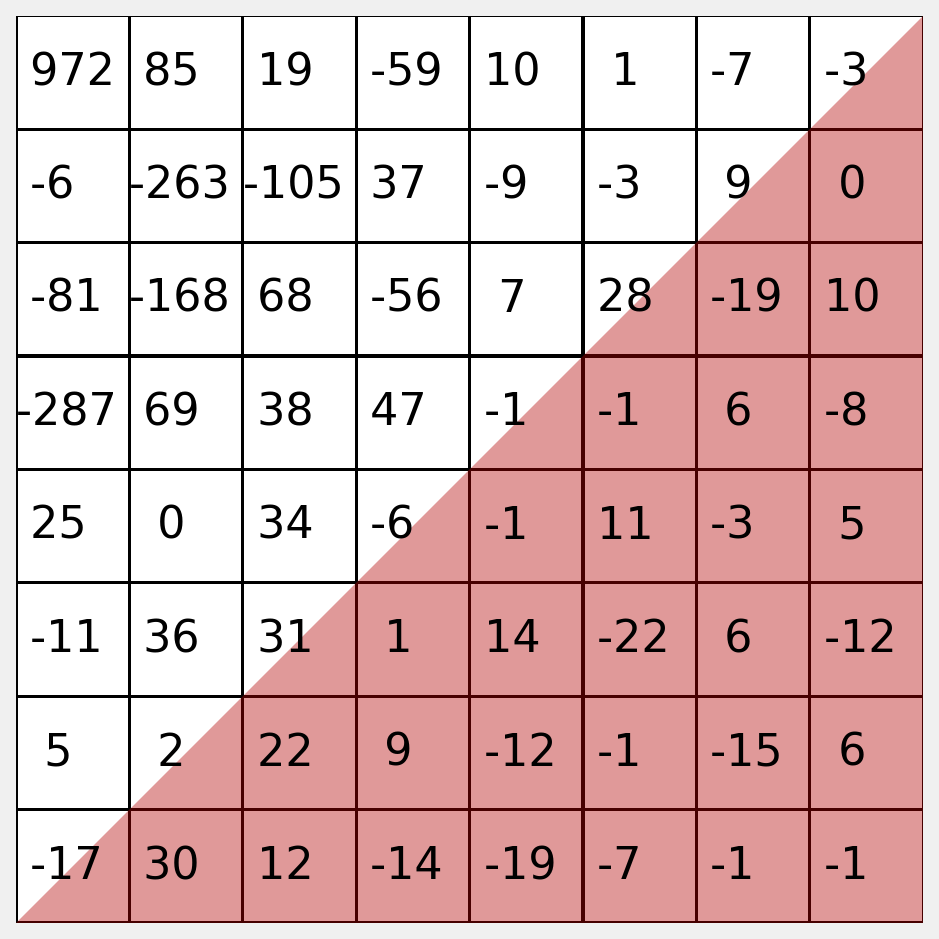
If we want to reconstruct the image using the inverse DCT, we can set the low values to zero to view the reconstruction loss.

DCT for 2D Signals

Here you can see we have zeroed the lower right triangle.

You should decide empirically how many coefficients to retain. Often, many fewer than half produce good results.

DCT Features

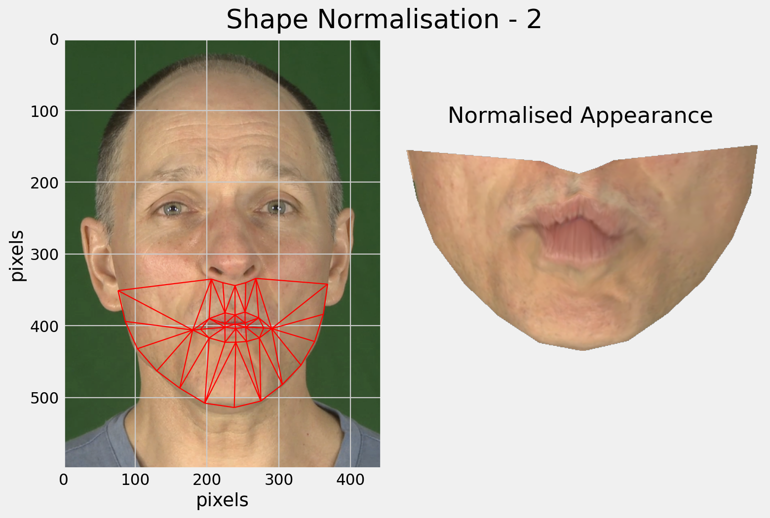
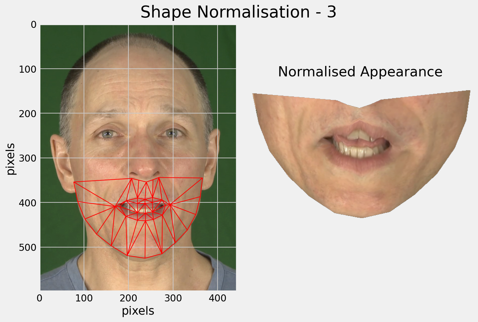
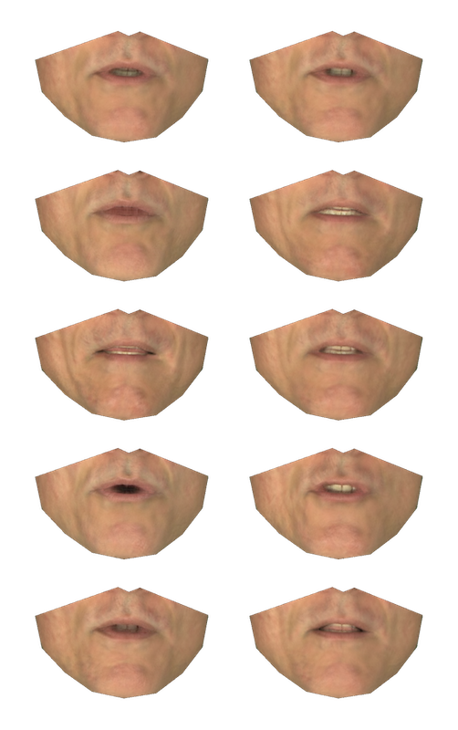
One approach for modelling the appearance of the face:

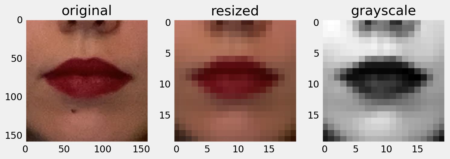
Convert the image to greyscale.
Crop the image to contain only the region of interest (the mouth).
Normalise the size of the image to some default size (the images need the same number of pixels in each frame).
Either resize the cropped regions, or better, use a constant clipping box.

DCT Features

One approach for modelling the appearance of the face:

Segment the region into n x n pixel blocks.
Experiment with \(1 \leq n \leq 8\).
Apply a 2D Discrete Cosine Transform (DCT) to each block.
Extract coefficients that encode low frequency information.

2D DCT case study

A region of interest is cropped, resized and converted to greyscale.

2D DCT case study

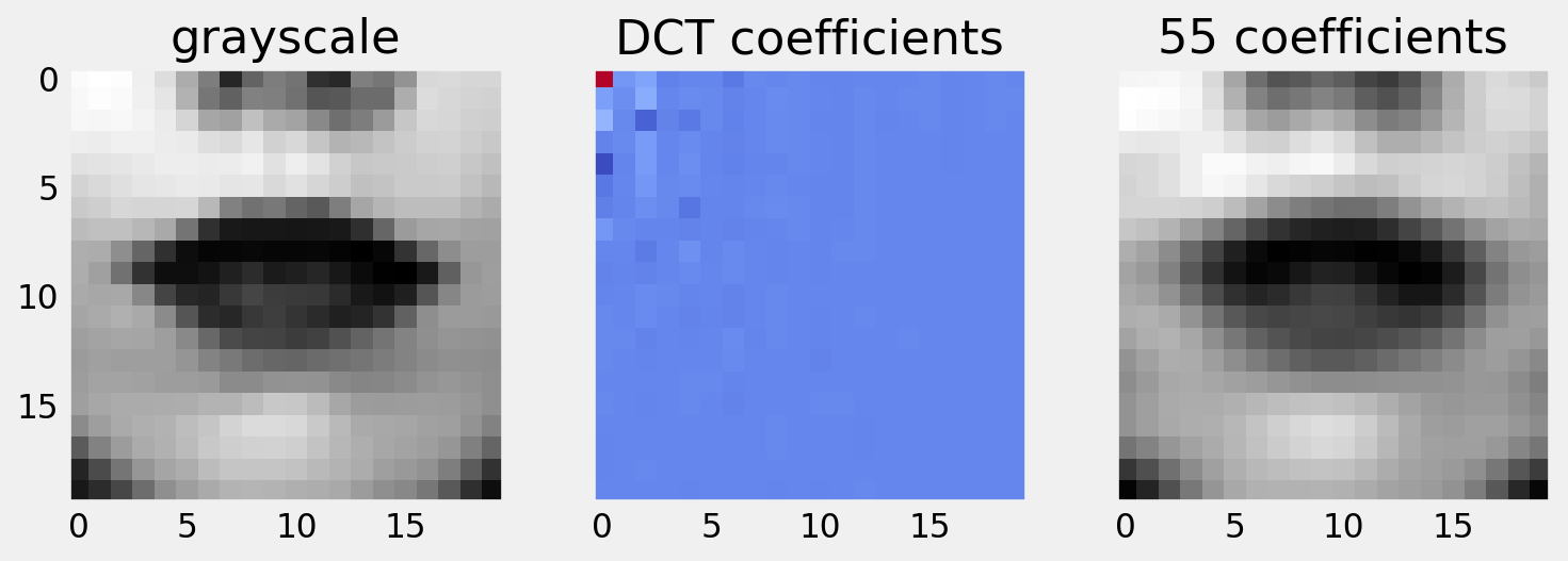
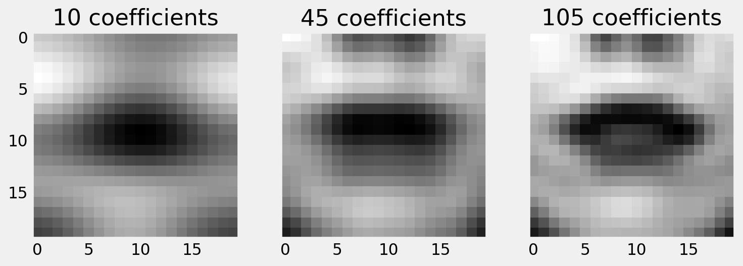
From the greyscale image, we can extract the DCT coefficients. We retain only the low frequency coefficients, and show a reconstruction of the image.

2D DCT case study

Perceptual evaluations of the reconstruction are informative, but your experiments should determine how useful the features are for recognising speech.

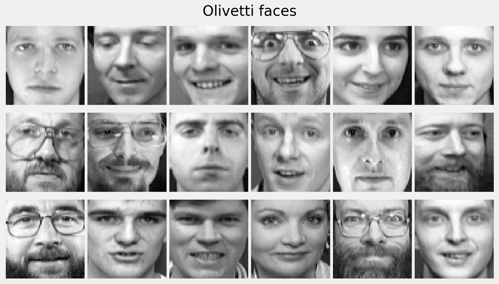
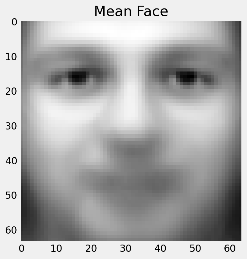
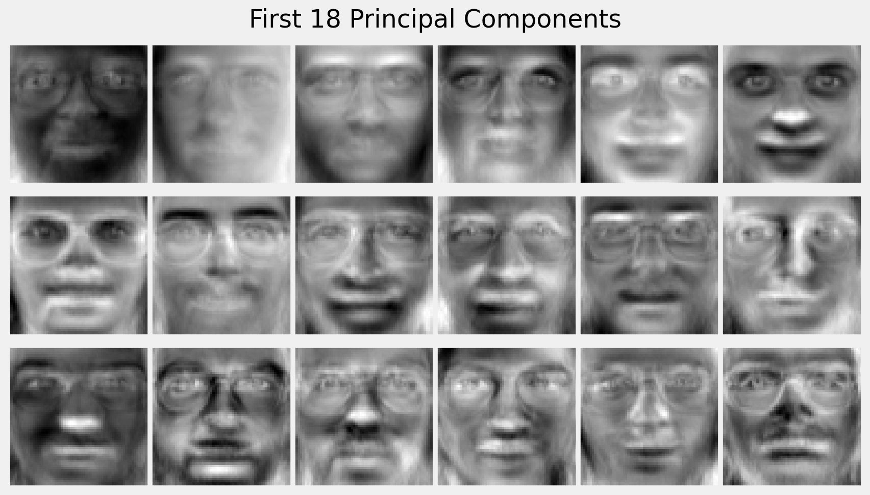
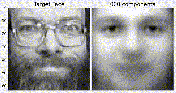
Eigenfaces

Crop the images to contain only the region of interest.
Normalise the size of the image.
Images need the same number of pixels in each frame.
Resize the images, or better, use a constant clipping box.

Eigenfaces

Apply PCA to the size-normalised images.
When applied to face images, referred to as Eigenfaces.
This was the basis of an early face recognition system. (Turk and Pentland, 1990).

Eigenfaces

Training data is the Olivetti Faces corpus.

Eigenfaces

Recall, to reconstruct using PCA:

\[\mathbf{x} \approx \mathbf{\overline x} + \mathbf{P} \mathbf{b}\]

Eigenfaces

A human face can be approximated from the mean shape plus a linear combination of the eigenfaces.

Eigenfaces

Eigenfaces

Appearance Models

There is problem with the Eigenface approach:

There are two sources of variation - shape and appearance.
One model is trying to capture both.
We see ghosting in the images when reconstructed.

Appearance Models

We should model only the appearance variation.

A PDM is already able to model the shape.

Appearance Models

Each pixel should represent the same feature.

We can’t achieve this goal by merely normalising the crop.

Appearance Models

Given the hand-labelled images that were used to build the PDM, warp the images from the hand labels to the mean shape.

There are many ways to perform the warp, e.g.:

Triangulate the landmarks, then map the pixels accordingly.

Appearance Models

For each image in the training data, and for each triangle:

Find \(M\) for \(MA = B\), where \(A\) is a triangle in an image and \(B\) is the corresponding triangle in the mean shape.
Use \(M\) to warp the pixels in each triangle.
Accumulate the patches into one shape normalised image.

Appearance Models

Images are shape-normalised.

They all have the same number of pixels.
Each pixel represents the same feature.

Appearance Models

Applying PCA to the shape-normalised images gives a better model of appearance.

The shape model and the appearance model can be combined or concatenated.
The appearance can provide a photo-metric loss for model fitting.

Effectiveness of Visual Features

Effectiveness

Potamianos et al. (1998) compared visual features for automatic lip-reading.

They trained models for a single talker reciting connected digits and measured accuracy as % correct.

Effectiveness

Feature Class	Feature	Accuracy
Articulatory	Height and Width	55.8%
	and Area	61.9%
	and Perimeter	64.7%
Fourier Descriptors	Outer Lip Contour	73.4%
	Inner Lip Contour	64.0%
	Both Contours	83.9%
Appearance	LDA - based features	97.0%

Effectiveness

Lan et al. (2010) compared visual features for automatic lip-reading.

Appearance (app)
PDM (shape)
DCT (2ddct)
Eigenface (eigen-lip)
Shape and Appearance (aam-pca)

Model Fusion

Audiovisual Fusion

The acoustic and visual information needs to be combined - how and where this happens is important.

We require that the performance after fusion is not worse than best performing individual modality.

Audiovisual Fusion

Two strategies:

Early integration: fusion is prior to recognition, e.g. at the feature level.
Late integration: fusion is after recognition, e.g. sentence-level.

Audiovisual Fusion

Usually an estimation of the respective confidence is required.

Could be fixed, where it is learned during training based on accuracy.
Could be adaptive, where it reflects the noise in the respective channels.

Early Integration

Advantage of early integration:

We can simply concatenate the features.
The structure of the recogniser does not need to change.

Early Integration

Disadvantages of early integration:

Size of the feature vector increases making training more difficult.
Need to normalise the features from different modalities, or weight them appropriately
Acoustic noise affects all of the input feature vectors.
Need to worry about the data rate, which might be different for both modalities.

Late Integration

Advantages of late integration:

Acoustic noise will not affect the visual recogniser.
Easier to adapt the recogniser to different conditions.
Notionally less training data are required to train the respective models.
Extends the structure of existing recognisers.
Either fuse the outputs or use a multi-stream HMM.

Late Integration

Disadvantages of late integration:

May need to worry about the data rate, which is different for both modalities
Introduces extra parameters to optimise during training.

Summary

Integrating visual information can improve the robustness of speech recognisers to acoustic noise.

Face encoding using:

DCT Features
Eigenfaces
Appearance Models