Content
Lossy and lossless image compression.
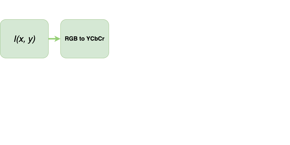
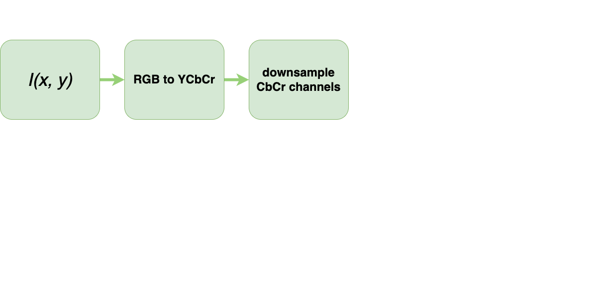
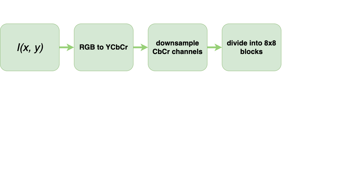
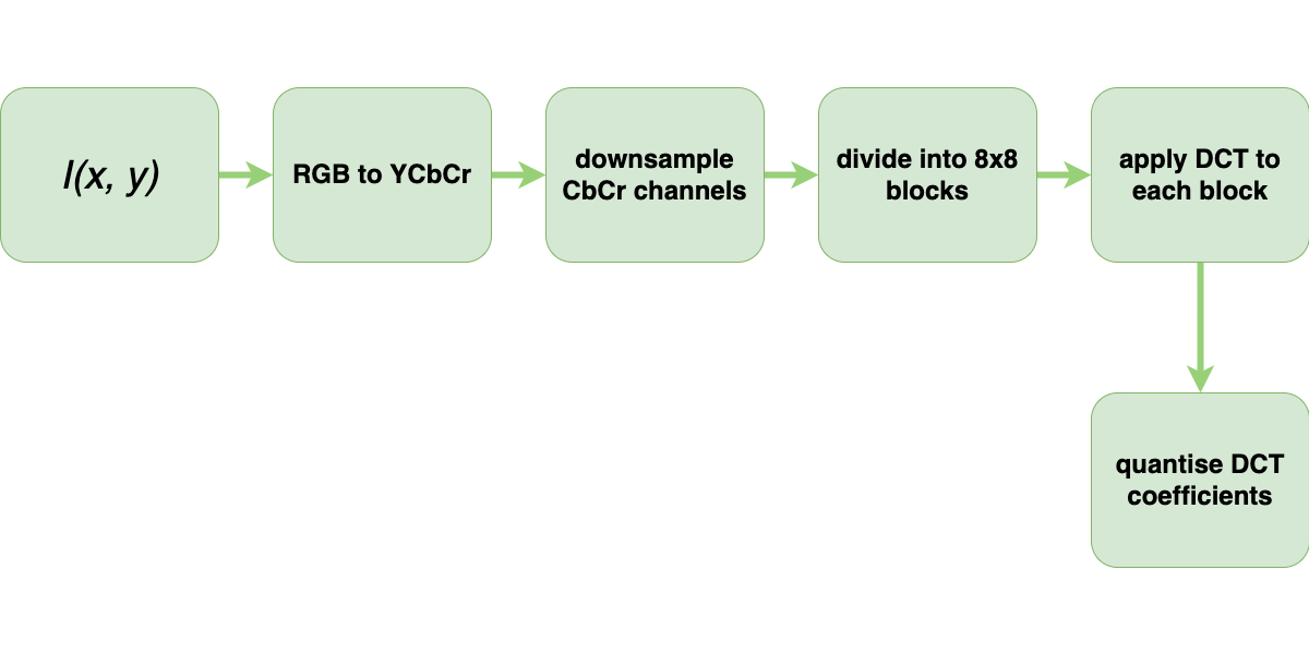
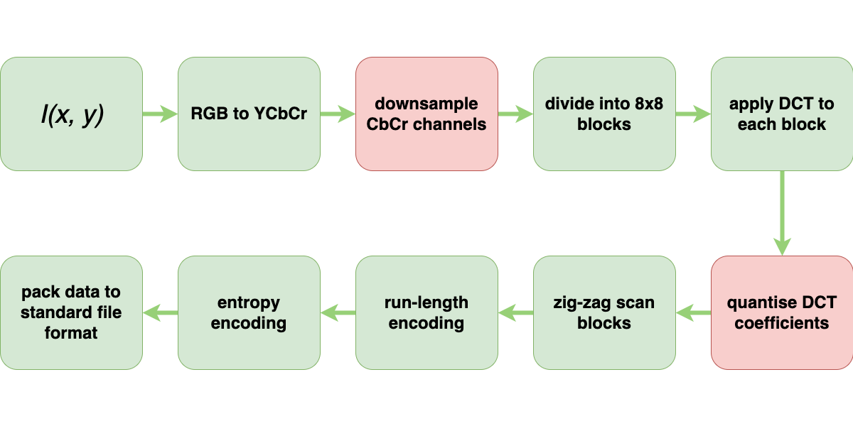
- Changing colour spaces and subsampling
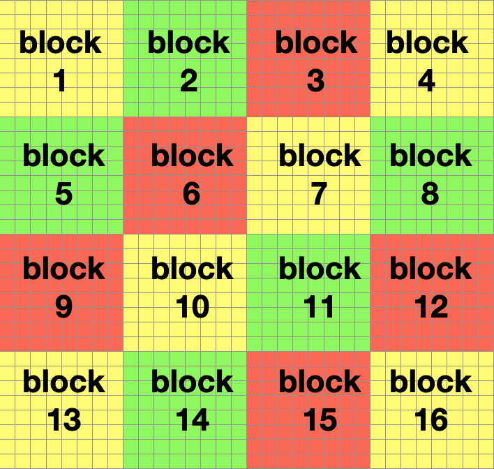
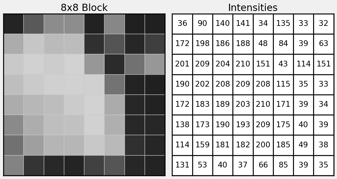
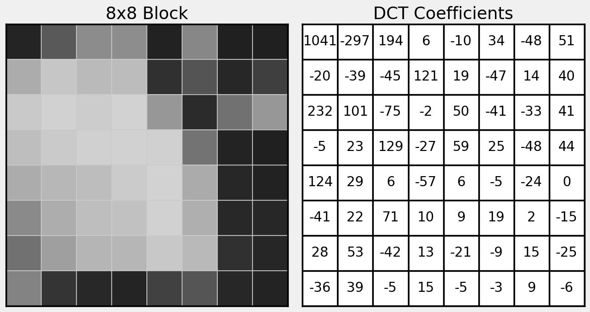
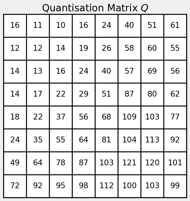
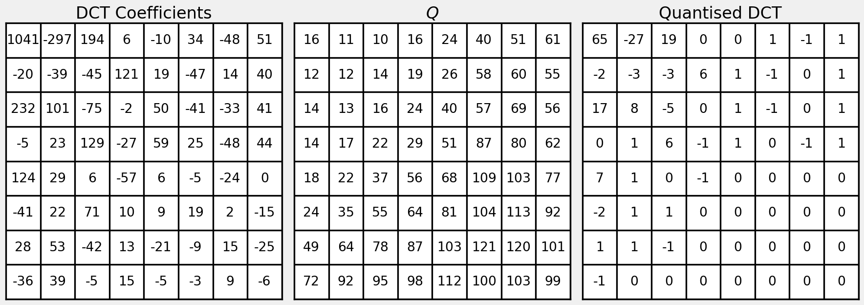
- DCT and quantisation
- Run-length encoding
- Entropy coding
Run Length Encoding
Extracts series of value and length of runs from sequence of values.
Exploits inter-pixel redundancy.
Run Length Encoding
65 -27 -2 17 -3 -3 1 1 1 -2 1 1 0 -1 1 0 0 0 0 0 0 0 0 0 0 0 0 0 0 0 0 0 0 0
Run Length Encoding
65 -27 -2 17 -3 -3 1 1 1 -2 1 1 0 -1 1 0 0 0 0 0 0 0 0 0 0 0 0 0 0 0 0 0 0 0
65 1 -27 1 -2 1 17 1 -3 2 1 3 -2 1 1 2 0 1 -1 1 1 1 0 19
Run Length Encoding
65 -27 -2 17 -3 -3 1 1 1 -2 1 1 0 -1 1 0 0 0 0 0 0 0 0 0 0 0 0 0 0 0 0 0 0 0
65 1 -27 1 -2 1 17 1 -3 2 1 3 -2 1 1 2 0 1 -1 1 1 1 0 19
Run Length Encoding
65 -27 -2 17 -3 -3 1 1 1 -2 1 1 0 -1 1 0 0 0 0 0 0 0 0 0 0 0 0 0 0 0 0 0 0 0
65 1 -27 1 -2 1 17 1 -3 2 1 3 -2 1 1 2 0 1 -1 1 1 1 0 19
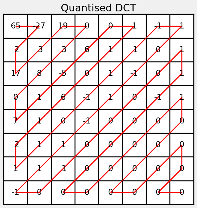
Run Length Encoding
65 -27 -2 17 -3 -3 1 1 1 -2 1 1 0 -1 1 0 0 0 0 0 0 0 0 0 0 0 0 0 0 0 0 0 0 0
65 1 -27 1 -2 1 17 1 -3 2 1 3 -2 1 1 2 0 1 -1 1 1 1 0 19
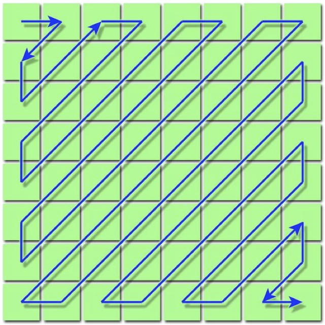
Run Length Encoding
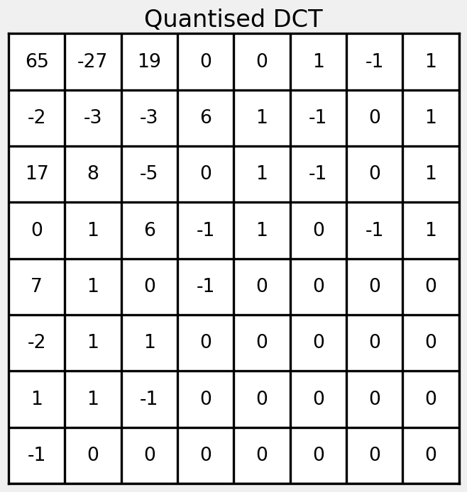
Exploits inter-pixel redundancy
- the relationship between neighbouring “pixels” in the zigzag scan of the DCT coefficient matrix
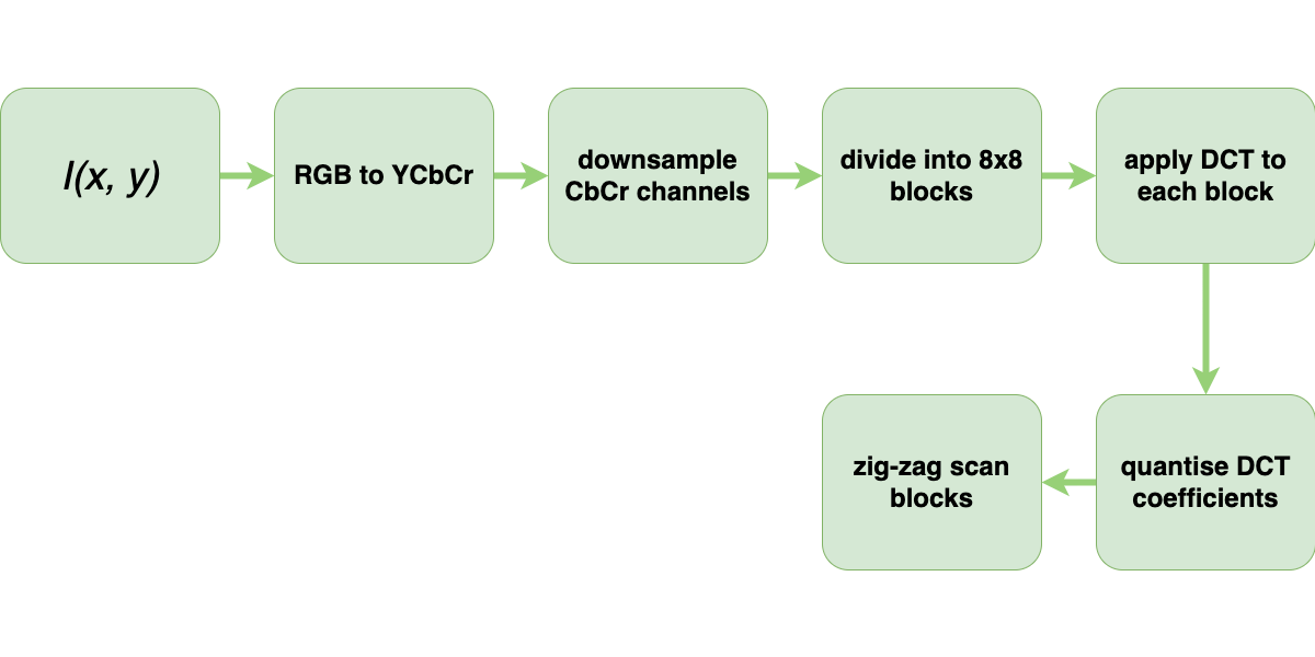
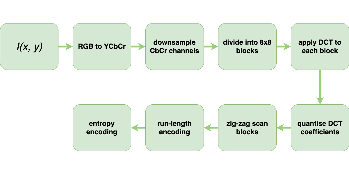
JPEG Compression
![entropy encoding]() entropy encoding
entropy encoding
Entropy Coding
Information and data are not the same thing.
- Claude Shannon, (1948). A Mathematical Theory of Communication.
Entropy Coding exploits coding redundancy
- not every value is equally likely.
Entropy Coding encodes a sequence with variable length code so that:
- More probable values have fewer bits, and
- less probable values have more bits.
The new alphabet requires fewer bits per pixel.
- How many bits do we need?
Recall: the probability of an event is:
\[p_{i} = \frac{N_{i}}{N}\]
The information in bits is:
\[I_{i} = - \log_{2} p_{i}\]
The entropy, the smallest possible mean symbol length, is:
\[H = - \sum_{i} p_{i} \log_{2} p_{i}\]
We can use these properties to develop a better coding for an image.
- The stream must be decoded unambiguously.
- One code cannot be the prefix of another.
Huffman Coding
Step 1:
- Arrange values in order of decreasing probability.
- Each forms a leaf in the Huffman tree.
Huffman Coding
Step 2:
- Merge the two leaves with the smallest probability,
- add the probabilities,
- insert the node into the sorted list.
- Assign a 1/0 to each branch being merged.
Huffman Coding
Step 3:
- Repeat until only the root node remains.
- Read codewords from the root to the leaves.
Huffman Coding
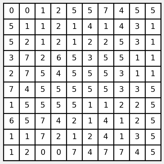
What is the Huffman code for this image?
And, what is the current bit rate?
Count the frequencies of each symbol.
| 4 |
0 |
| 23 |
1 |
| 15 |
2 |
| 8 |
3 |
| 10 |
4 |
| 29 |
5 |
| 2 |
6 |
| 9 |
7 |
What is the entropy of this image?
| 0.29 |
1.786 |
0.518 |
| 0.23 |
2.120 |
0.488 |
| 0.15 |
2.737 |
0.411 |
| 0.10 |
3.322 |
0.332 |
| 0.09 |
3.474 |
0.313 |
| 0.08 |
3.644 |
0.292 |
| 0.04 |
4.644 |
0.186 |
| 0.02 |
5.644 |
0.113 |
|
\(+\) |
2.651 |
Sort by the most frequent symbol.
| 29 |
5 |
| 23 |
1 |
| 15 |
2 |
| 10 |
4 |
| 9 |
7 |
| 8 |
3 |
| 4 |
0 |
| 2 |
6 |
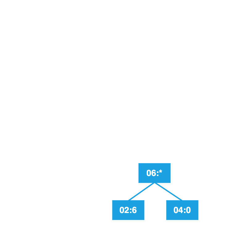
Merge the two leaves with the lowest frequency…
![]()
Insert the node into the sorted list.
| 29 |
5 |
| 23 |
1 |
| 15 |
2 |
| 10 |
4 |
| 9 |
7 |
| 8 |
3 |
| 6 |
* |
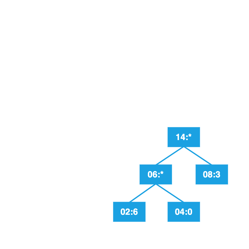
Repeat with the next two lowest frequencies.
![]()
Insert the node into the sorted list.
| 29 |
5 |
| 23 |
1 |
| 15 |
2 |
| 14 |
* |
| 10 |
4 |
| 9 |
7 |
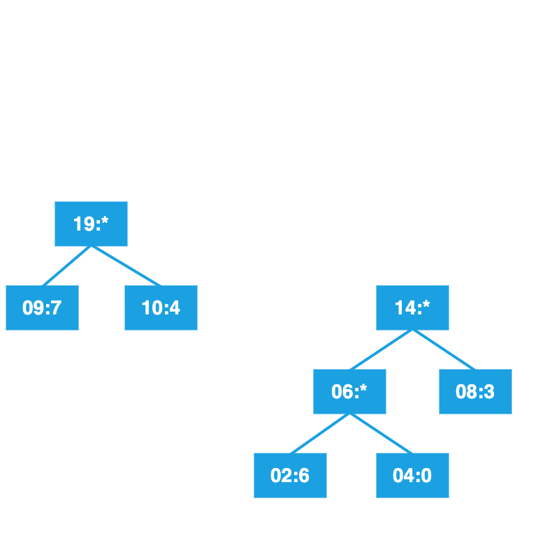
Repeat with the next two lowest frequencies.
![]()
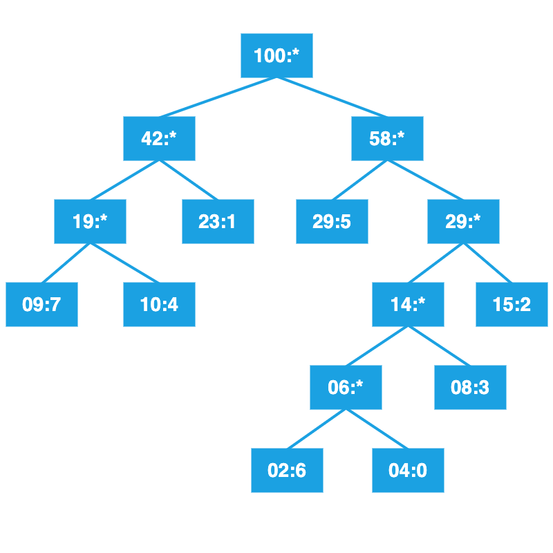
Continue until the tree is complete.
![]()
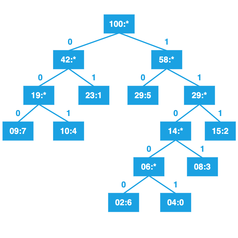
Label left branches with 0, right branches with 1.
![]()
Read from the root to compute the new codes.
| 11001 |
0 |
| 01 |
1 |
| 111 |
2 |
| 1101 |
3 |
| 001 |
4 |
| 10 |
5 |
| 11000 |
6 |
| 000 |
7 |
| 5 |
0.29 |
2 |
0.58 |
| 1 |
0.23 |
2 |
0.46 |
| 2 |
0.15 |
3 |
0.45 |
| 4 |
0.10 |
3 |
0.30 |
| 7 |
0.09 |
3 |
0.27 |
| 3 |
0.08 |
4 |
0.32 |
| 0 |
0.04 |
5 |
0.20 |
| 6 |
0.02 |
5 |
0.10 |
|
|
+ |
2.68 |
We can calculate the bit rate we achieved.
- Not optimal.
- optimal bit rate is \(2.65\)
- our bit rate is \(2.68\)
- The compression ratio is \(2.68/3.0 = 0.8933\).
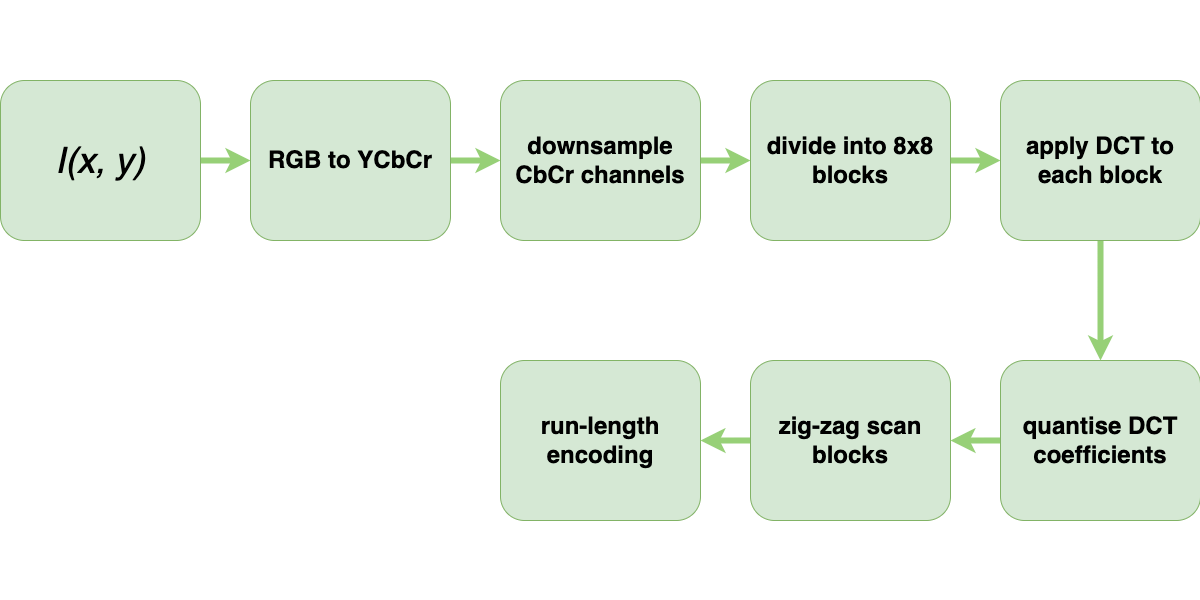
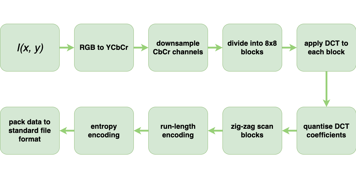
JPEG Compression
![data packing]() data packing
data packing