Content
- Introducing Images
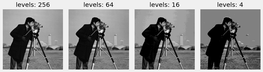
- Sampling and Quantisation
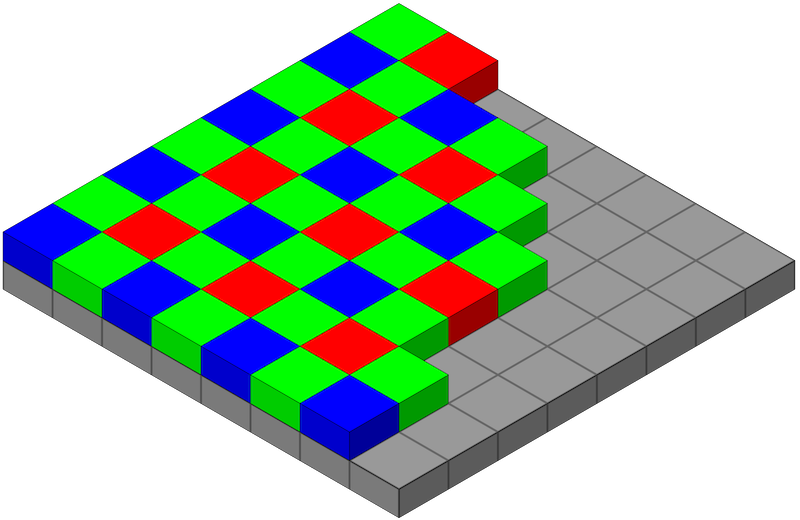
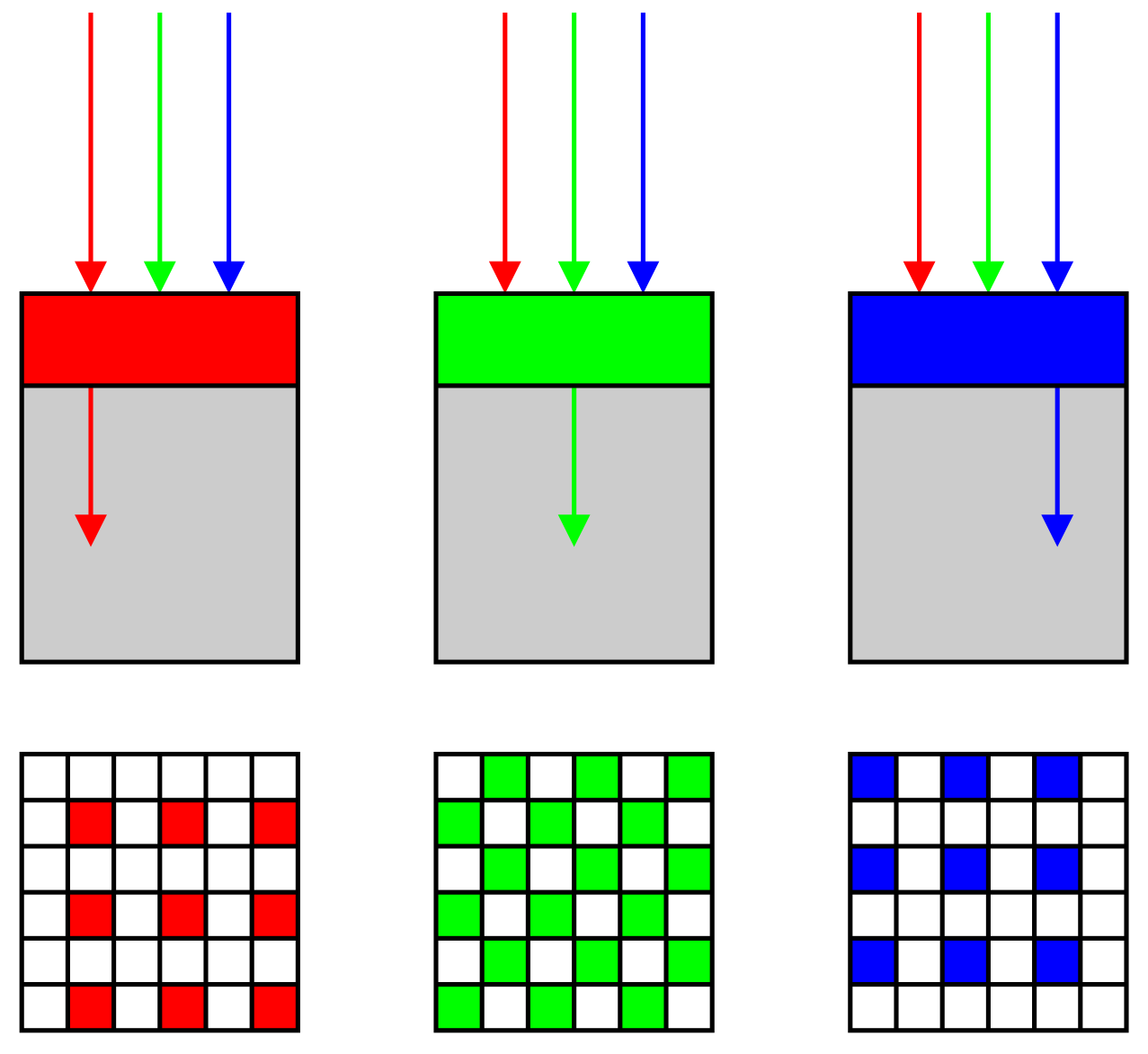
- Image Capture
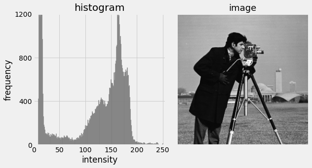
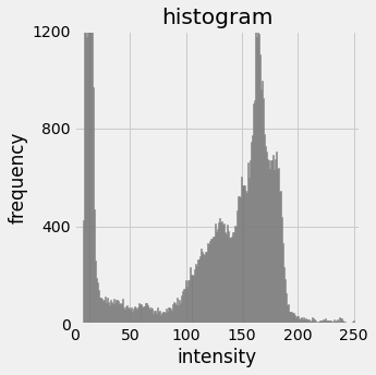
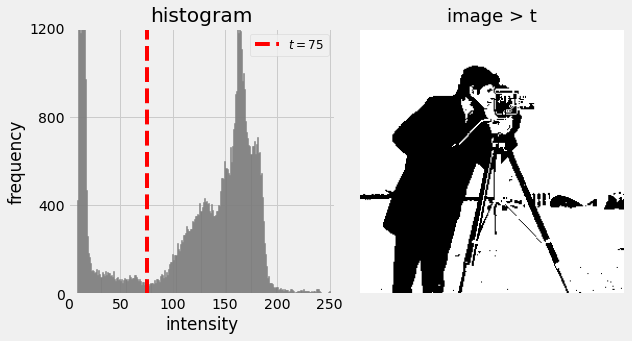
- Controlling and Analysing Images
- Video
Audiovisual Processing CMP-6026A
Dr. David Greenwood
Arguably the most important scientific instrument to date, practical photography with a camera arrived in 1839.
Simultaneously claimed by Louis Daguerre and William Henry Fox Talbot, and preceded by far less useful solutions.
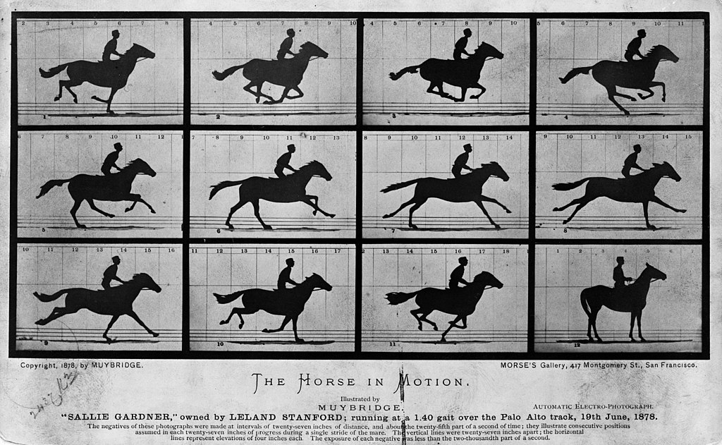
Proved a galloping horse lifts all four hooves off the ground at one point in its sequence of motion.
Perhaps the earliest movie?
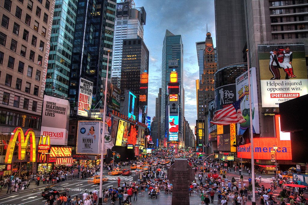
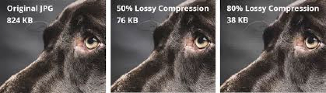
Efficiently describe complex information…
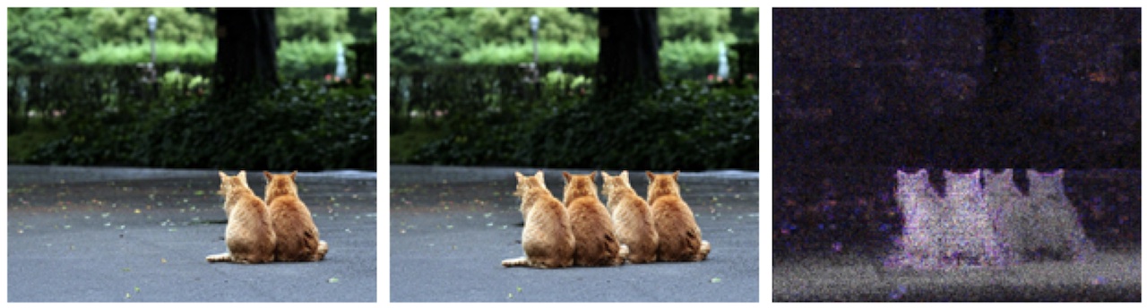
Image data can contain data other than photographs.
How do we represent images on a computer?
Colour images can be defined as a set of functions:
In order to become suitable for digital processing, an image function \(f(x,y)\) must be digitized both spatially and in amplitude.
To digitise an image we discretise it by sampling spatially on a regular grid.
The number of samples determines the resolution of the image.
A pixel (picture element) at \((x,y)\) is the image intensity at the grid point indexed by the integer coordinate \((x,y)\).
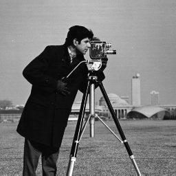
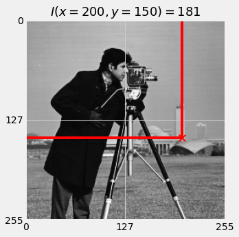
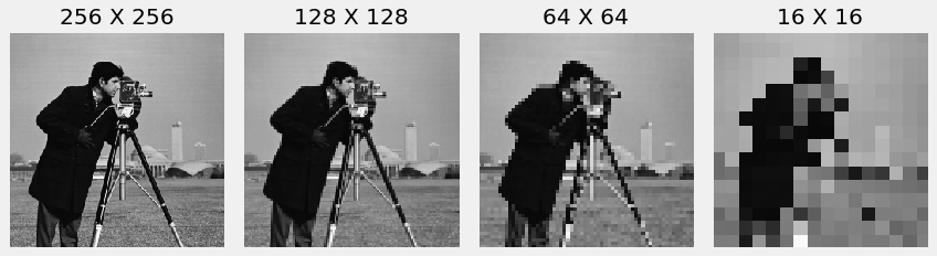
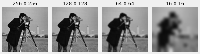
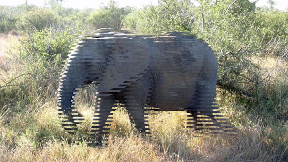
We can sample the image at various resolutions.
NOTE: Here we use bi-cubic interpolation to display the images.
You have already encountered sampling in the context of audio.
In audio the real signal is in the time domain.
For images, the real signal is in the spatial domain.
Transform a real-valued sampled image to one that takes a finite number of distinct values.
A pixel is usually represented by 8 bits, representing 256-levels.
Digital Photography
Colour is not a physical phenomenon - it is how humans perceive light of different wavelengths (analogous to perception of frequency in audio waveforms)
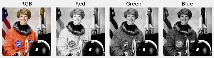
Visible spectrum and receptor response for “normal” vision.
Wavelengths perceived as green trigger both M and L cone cells in the eye.
Abnormalities in the cone response leads to colour blindness.
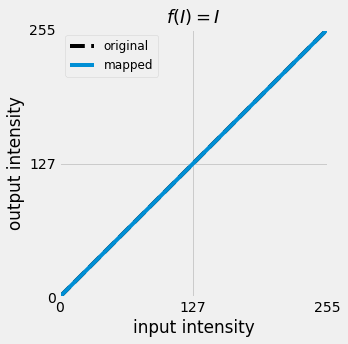
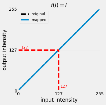
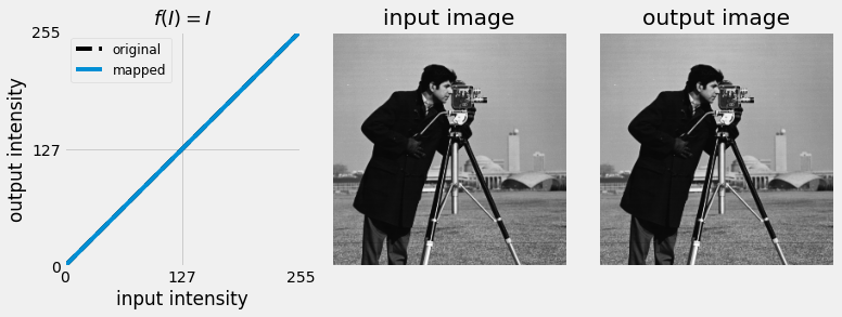
Exposure controls the brightness of an image.
Adjust shutter speed and aperture size to control the amount of light reaching the image sensor.
Adjust with a tone curve; a mapping from input to output pixel intensity.
As a linear function
Beware of implicit type conversion in your code.
\[f(I) = I\]
\[f(I) = I\]
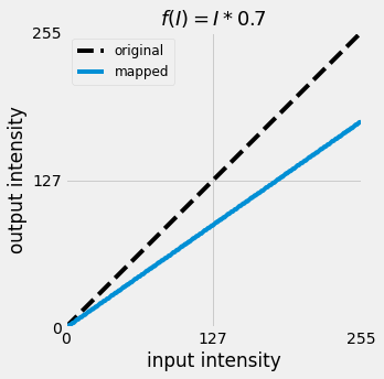
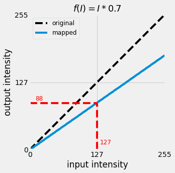
\[f(I) = I \times 0.7\]
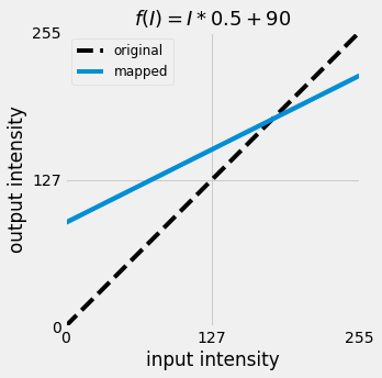
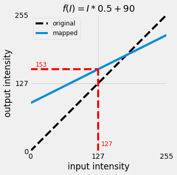
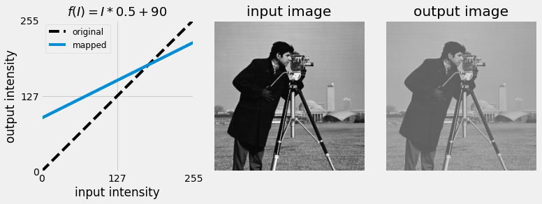
\[f(I) = I \times 0.5 + 90\]
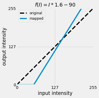
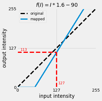
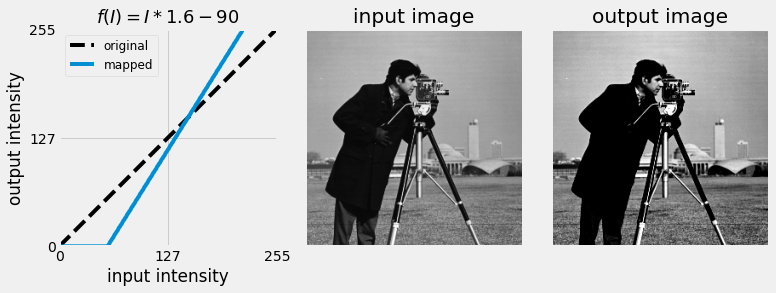
\[f(I) = I \times 1.6 - 90\]
Our eyes perceive brightness on a logarithmic scale.
Similar to how we perceive loudness in audio.
We have more cells that see in dim light than those that see in bright light.
We are more sensitive to low light changes.
Cameras measure light on a linear scale.
Tone curves can be used to adjust images so that they more closely match human perception of a scene.
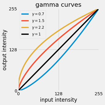
\[I^{\prime} = 255 \times \frac{I}{255}^{\frac{1}{\gamma}}\]
A histogram is an approximate representation of the distribution of numerical data.
We want to show the frequency, or count, of the values in an image.
Thresholding is the simplest method of segmenting images.
If we wanted to separate the coat from the sky, we could use a threshold.
By observing the histogram we could separate all pixels above or below a value.
\[I_{t} = I > t\]
We can consider video as a sequence of consecutive images.
The rate at which images are captured - or displayed.