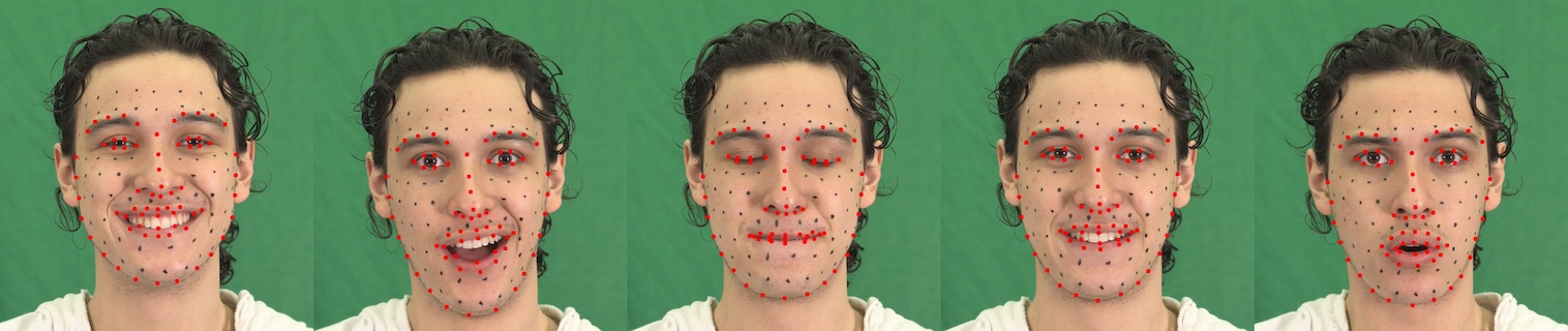
The consistency in the labelling ensures the elements of these vectors have the same meaning.
Point Distribution Models
The coordinates describe the shape in the image coordinate frame.
The same shape at different locations results in a different shape vector.
Point Distribution Models
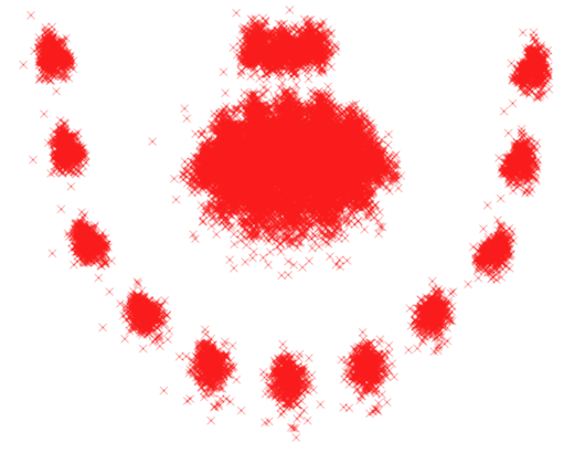
We need to normalise shapes for translation, scale and rotation. This can be done using Procrustes analysis.
Aside: Procrustes analysis
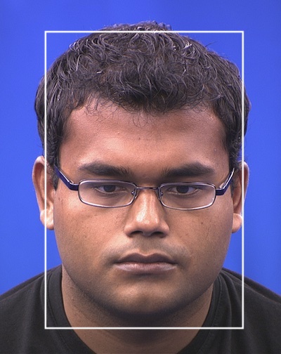
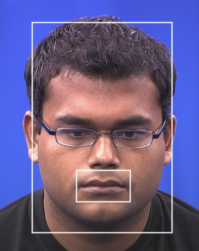
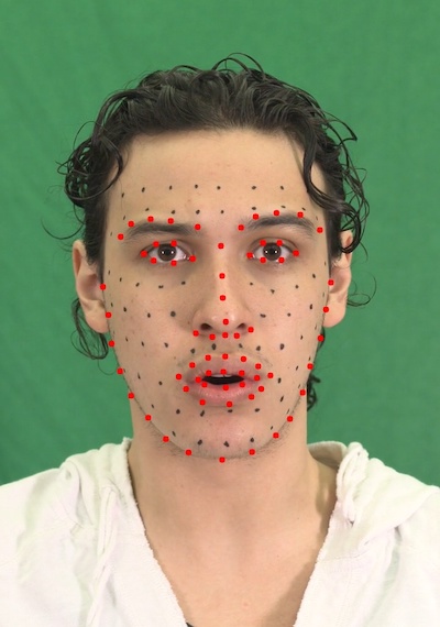
captured landmarks
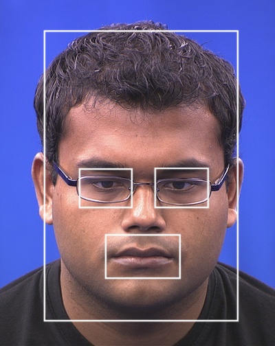
aligned landmarks
Point Distribution Models
Given the aligned shapes, compute a model that describes the variation in shape.
A linear model of the variation can be found using Principal Components Analysis (PCA).
Point Distribution Models
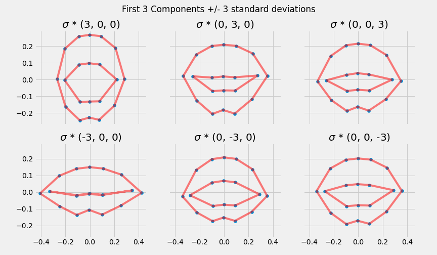
The model is in the form:
\[x = \overline x + \mathbf{P}_{s} \mathbf{b}_{s}\]
where \(x\) is a shape, \(\overline x\) is the mean shape, the matrix \(\mathbf{P}_{s}\) describes the variation in shape, and \(\mathbf{b}_{s}\) are the parameters that represent a shape instance.
Aside: Principal Component Analysis (PCA)
Reveals the internal structure of the data in a way that best explains the variance in the data.
Used for dimensionality reduction.
Reduces data down into its basic components, stripping away any unnecessary parts.
Aside: Principal Component Analysis (PCA)
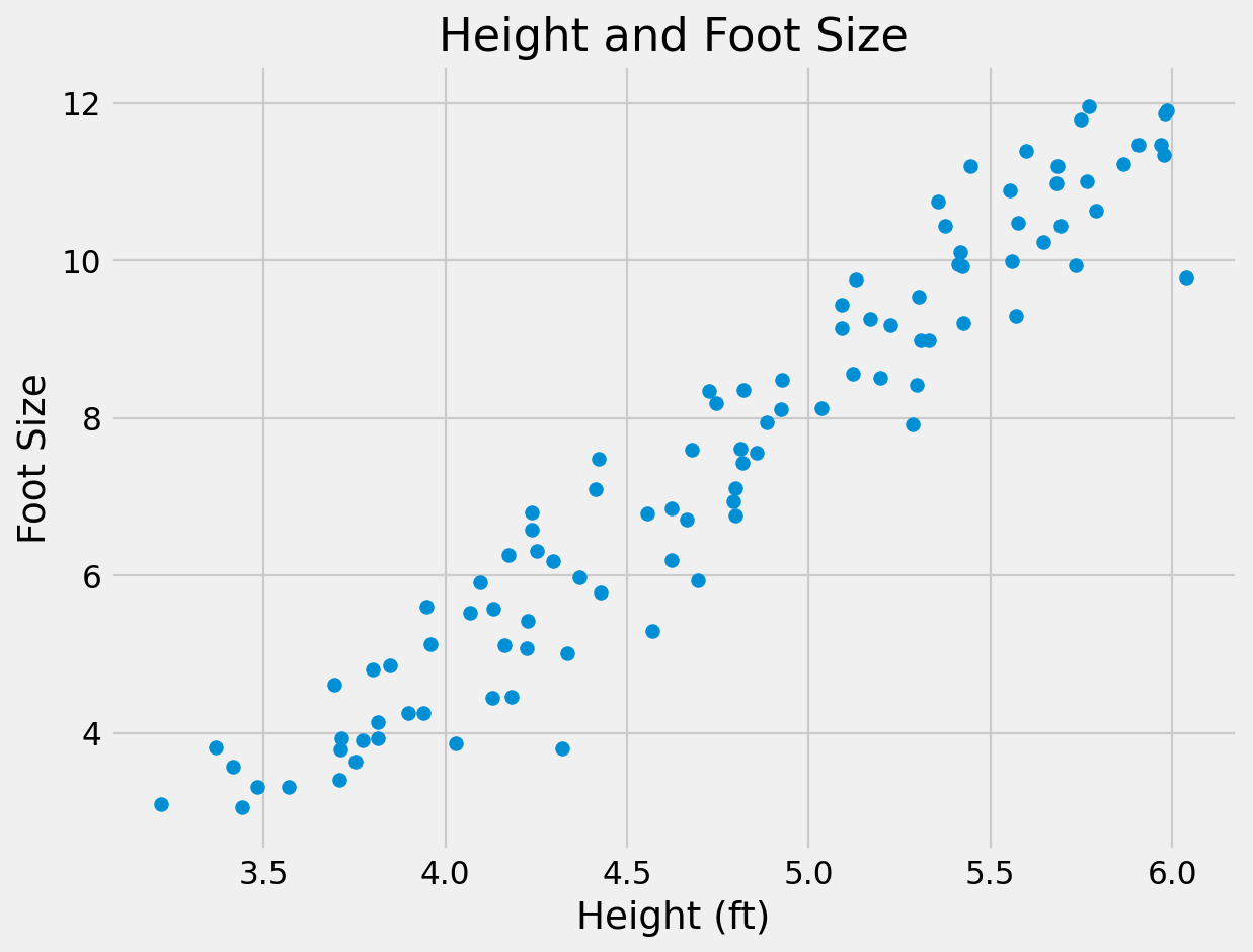
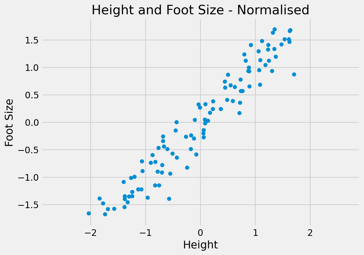
Assume we have 2-dimensional measurements. e.g. the height and foot size for a number of people
We expect the measurements to be correlated to some degree. e.g. taller people tend to have larger feet
Visualise the data by plotting one measure against the other.
Aside: Principal Component Analysis (PCA)
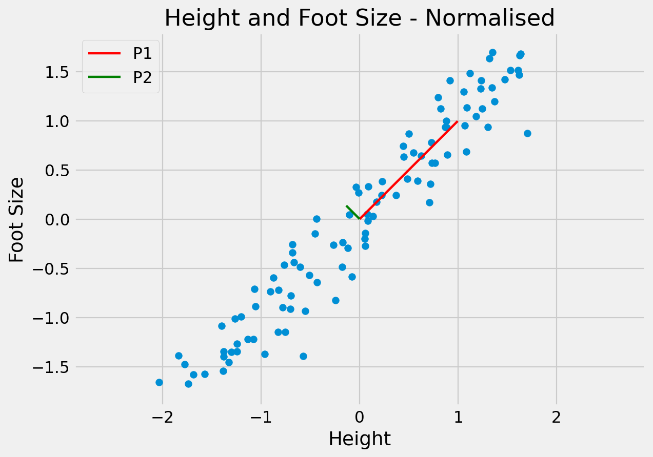
The objective of PCA is to capture as much of the variation in as few dimensions as possible.
Find line of “best fit” through the data, then line of “next best fit” which is orthogonal to the first…
Repeat for however many dimensions your data has
Aside: Principal Component Analysis (PCA)
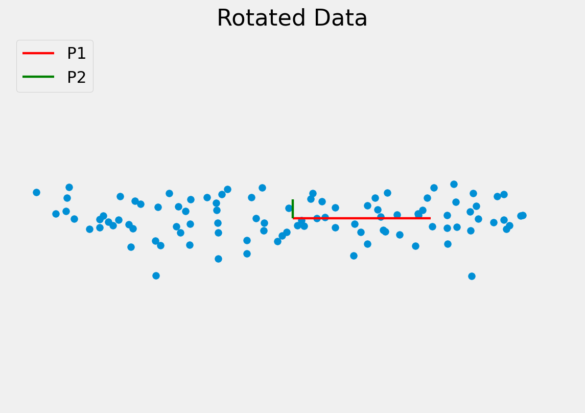
Since the dimensions must be orthogonal, all we have done is rotate the axes to better align with the data.
In doing this:
P1 captures most of the meaningful variation
P2 seems to capture the noise in the measurements
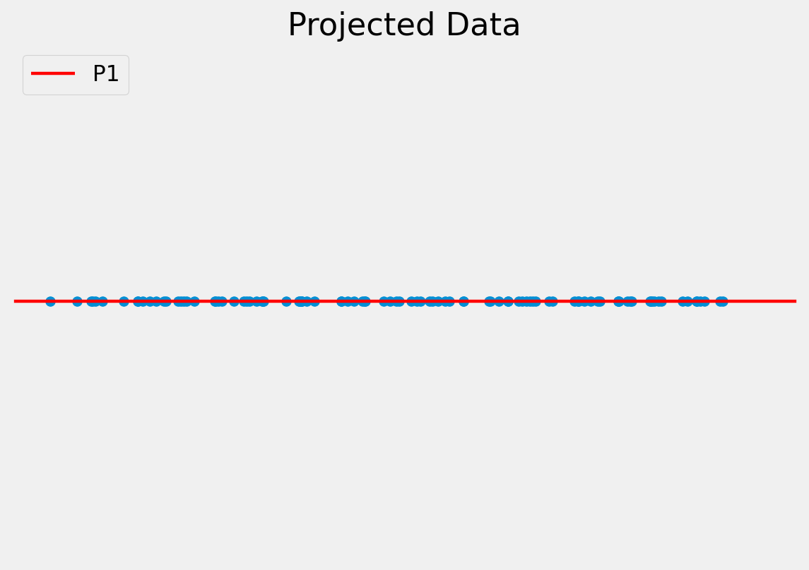
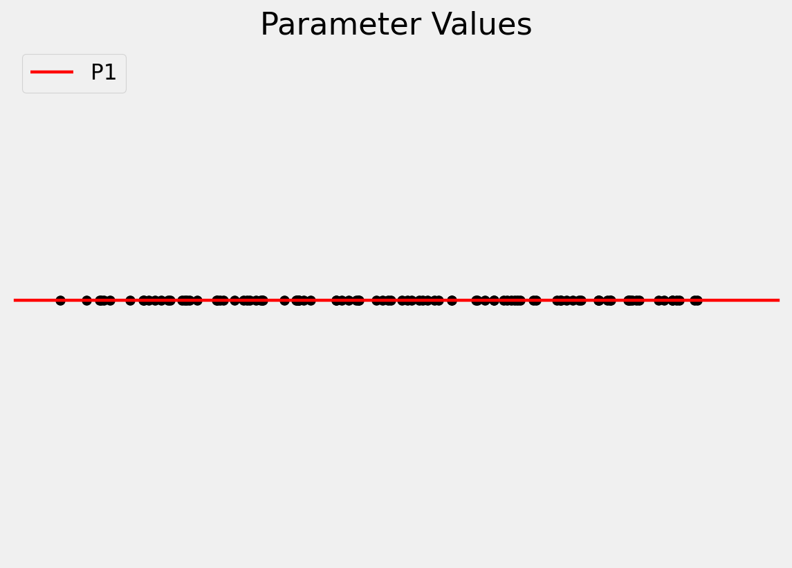
The original data can be approximated as some distance along P1 from the centre of the data cloud.
Aside: Principal Component Analysis (PCA)
To project a data point onto a new axis:
\[\mathbf{b}_{s} = \mathbf{P}_{s}^{T} (x - \overline x )\]
Aside: Principal Component Analysis (PCA)
To reconstruct the data point from the features:
\[x \approx \overline x + \mathbf{P}_{s} \mathbf{b}_{s}\]
This is only an approximation since the data are truncated to lie on just the principal component(s).
Aside: Principal Component Analysis (PCA)
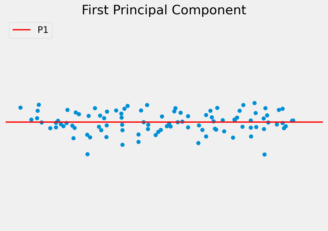
Note, in the previous example we have moved from a 2D problem to 1D so the representation is more compact.
Staying within the limits of the data means new examples can be generated — this is a generative model.
Aside: Principal Component Analysis (PCA)
Algorithm:
Compute the mean of the data and subtract.
Compute the covariance matrix.
Compute the eigenvectors and eigenvalues of the covariance matrix and sort into descending order of eigenvalue.
Aside: Principal Component Analysis (PCA)
Eigenvectors are the principal components.
Eigenvalues are the variance explained by each principal component.
We typically retain the number of eigenvectors that describe 95% of the total variation in the data.
Aside: Principal Component Analysis (PCA)
Matlab has implementations of both PCA and of Eigenvector/Eigenvalue decomposition.
Point Distribution Models
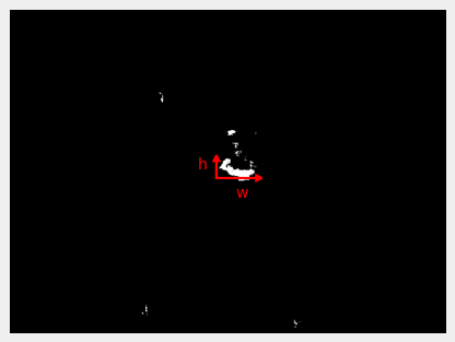
For modelling shapes, an n-point shape is represented as a 2n element vector: