Content
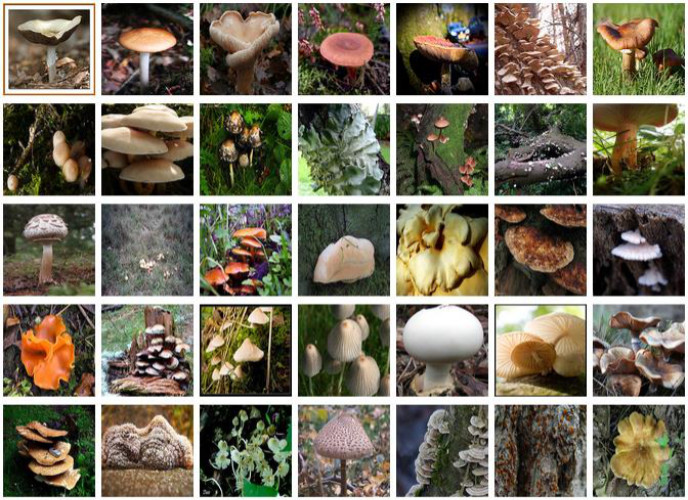
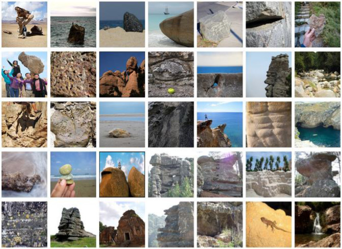
- ImageNet
- Neural Networks
- MNIST Examples
- Convolutional Neural Networks
Computer Vision CMP-6035B
Dr. David Greenwood
Spring 2022
\(> ~\) 1,000,000 images
\(> ~\) 1,000 classes
Actually…
\(> ~\) 15,000,000 images
\(> ~\) 20,000 classes
Ground truth annotated manually with Amazon Mechanical Turk.
Freely available for research here: https://www.image-net.org/
ImageNet Top-5 challenge:
You score if ground truth class is one your top 5 predictions!
Then the game changed!
In 2012, Krizhevsky et al. used a deep neural network to achieve a 15% error rate.
Prior approaches used hand designed features.
Neural networks learn features that help them classify and quantify images.
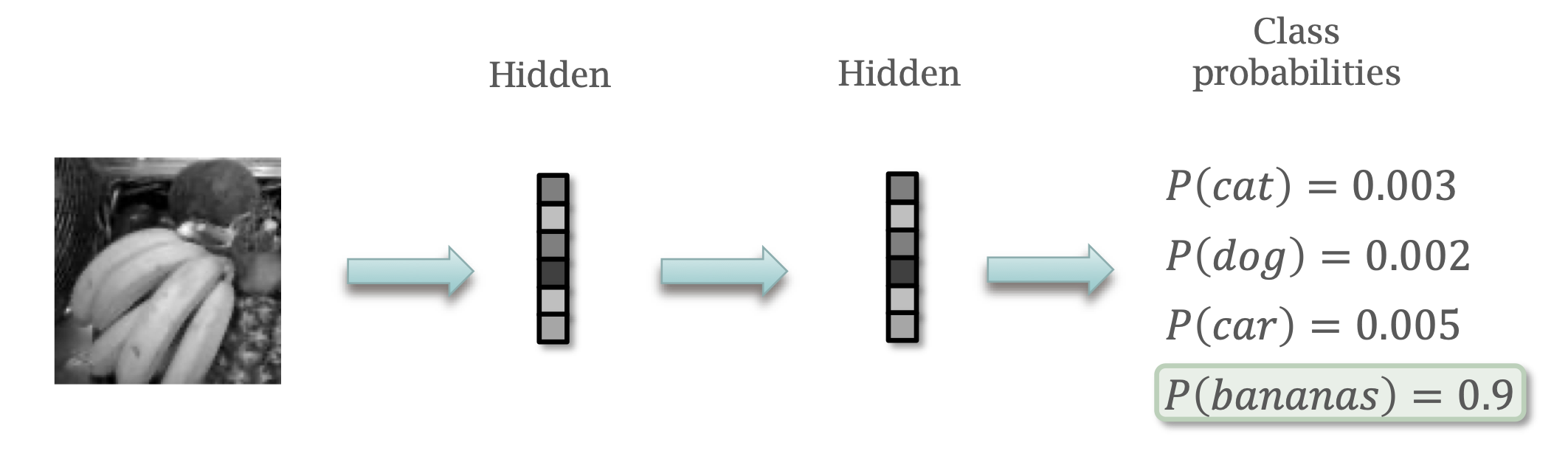
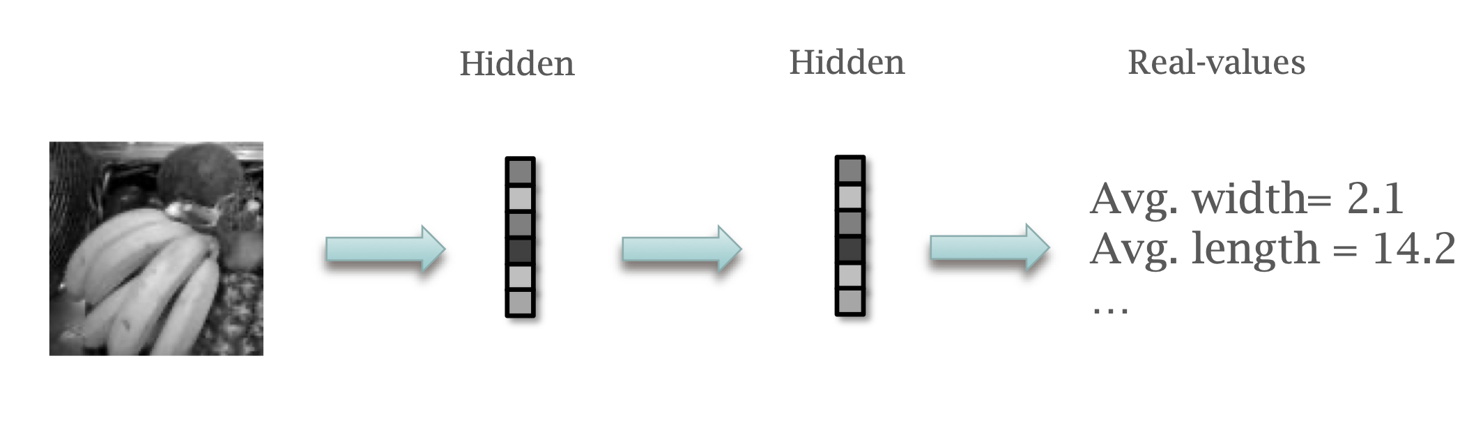
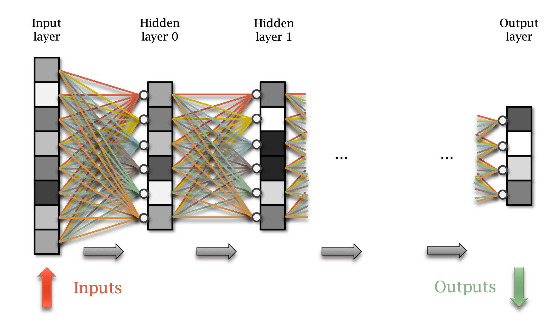
What is a neural network?
Multiple layers.
Data propagates through layers.
Transformed by each layer.
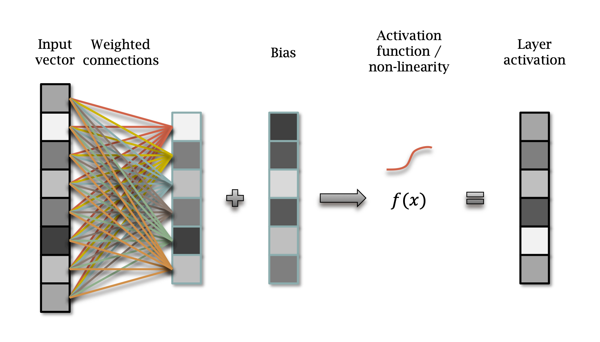
\[y = f(Wx + b)\]
\[y = f(Wx + b)\]
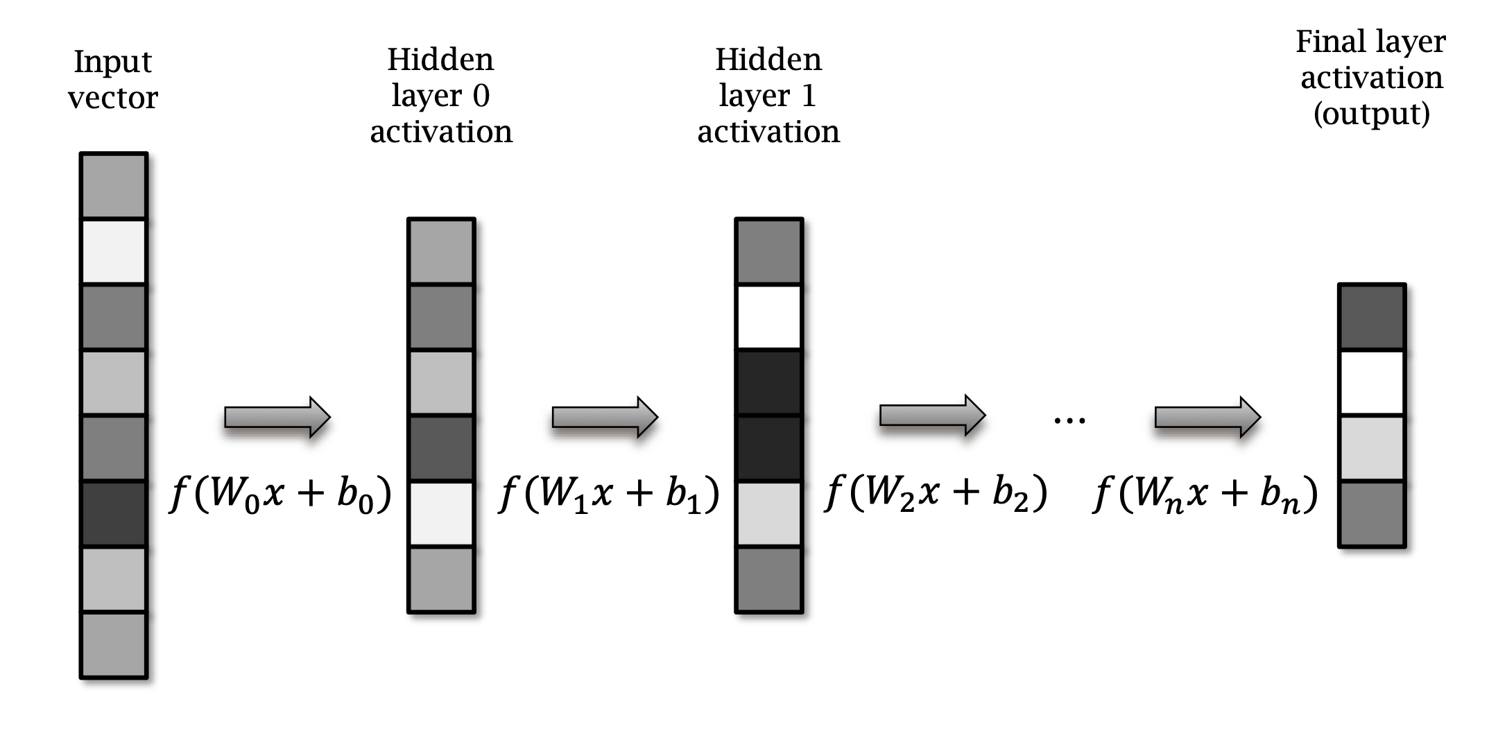
\[ \begin{aligned} y_0 &= f(W_0x + b_0) \\ y_1 &= f(W_1y_0 + b_1) \\ & \dotsc \\ y_L &= f(W_L y_{L-1} + b_L) \end{aligned} \]
A Neural Network is built from layers, each of which is:
… using PyTorch.
I’ve provided a small repository of code examples for you to try out, at:
https://github.com/uea-teaching/Deep-Learning-for-Computer-Vision
The first thing to note, is we usually work with batches of input data.
import torch, torch.nn.functional as F

# Assume input_data is S * M matrix
x = torch.tensor(input_data)

# W: gaussian random M * N matrix, std-dev=1/sqrt(N)
W = torch.randn(M, N) / math.sqrt(N)

# Bias: zeros, N elements
b = torch.zeros(1, N)

y = F.relu(x @ W + b)This is all a bit clunky.
PyTorch provides nice convenient layers for you to use.
# Assume input_data is S * M matrix
x = torch.tensor(input_data)

# Linear layer, M columns in, N columns out
layer = torch.nn.Linear(M, N)

# Call the layer like a function to apply it
y = F.relu(layer(x))On order to learn the correct weights, we need to train the model.
Define a cost to measure the error between predictions and ground truth.
Use back-propagation to modify parameters so that cost drops toward zero.
Initialise weights randomly.
For each example \(~x_{train}~\) from the training set.
Compute the derivative of cost \(~c\)
Update parameters \(W\) and \(b\) using gradient descent:
\[ \begin{aligned} W'_0 &= W_0 - \lambda \frac{\partial c}{\partial W_0} \\ b'_0 &= b_0 - \lambda \frac{\partial c}{\partial b_0} \\ \end{aligned} \]
\(\lambda\) is the learning rate: a hyperparameter.
Theoretically…use the chain rule to calculate gradients.
Many Neural Network tool-kits do all this for you automatically.
Write the code that performs the forward operations, PyTorch keeps track of what you did and will compute all the gradients in one step!
# Get predictions, no non-linearity
y_pred = layer(x_train)
# Cost is mean squared error
cost = ((y_pred - y_train) ** 2).mean()
# Compute gradients using 'backward' method
cost.backward()# Create an optimizer to update the parameters of layer
opt = torch.optim.Adam(layer.parameters(), lr=1e-3)
# Get predictions and cost as before
y_pred = layer(x_train)
cost = ((y_pred - y_train) ** 2).mean()
# Back-prop, zero the gradients attached to params first
opt.zero_grads()
# compute gradients
cost.backward()
# update the parameters
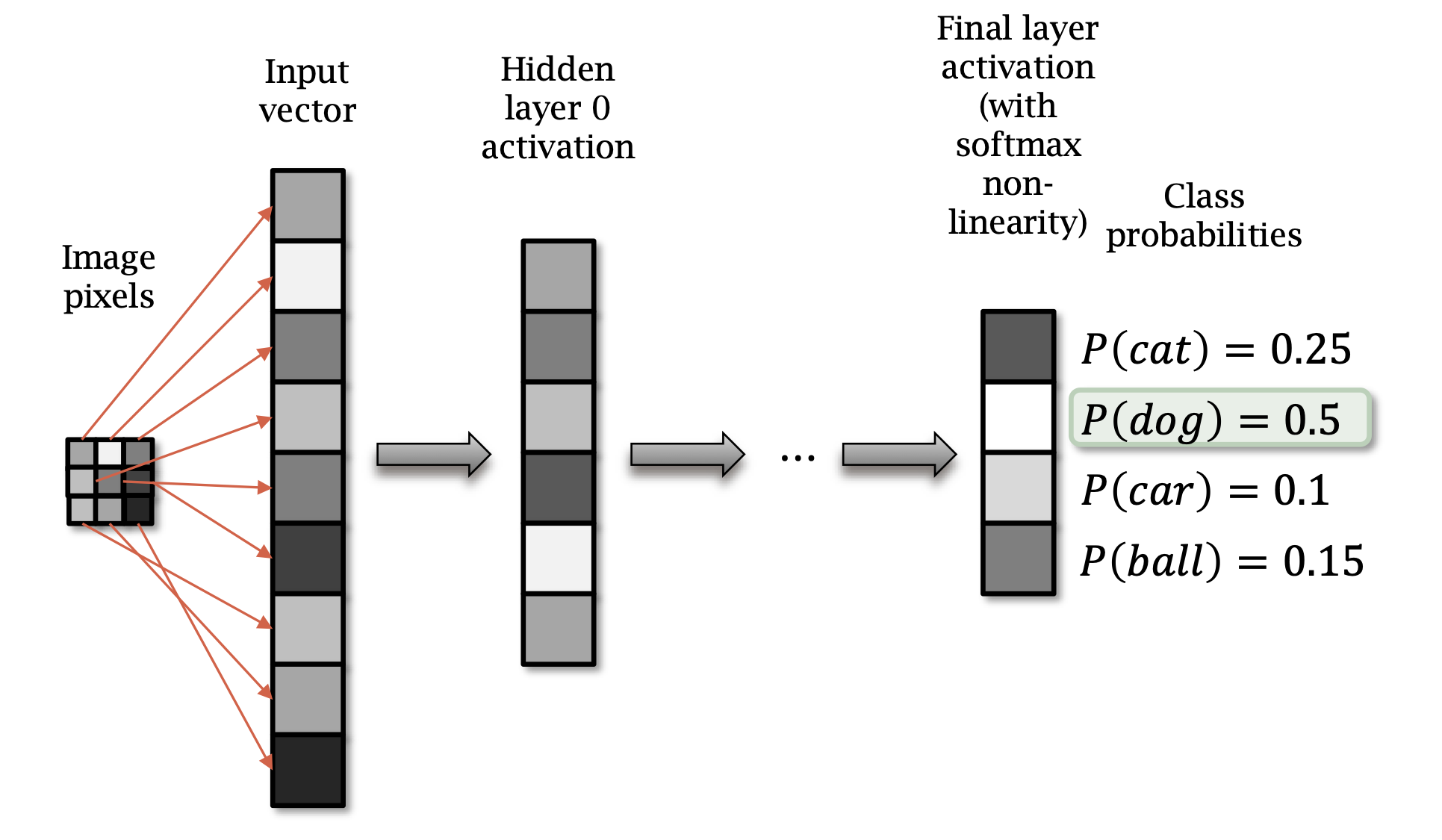
opt.step()Final layer has a softmax non-linear function.
The cost is the cross-entropy loss, which is the negative log-likelihood.
Softmax produces a probability vector:
\[ q(x) = \frac{e^{x_i}}{\sum_{i=0}^{N} e^{x_i}} \]
Negative log probability (categorical cross-entropy):
\[ c = - \sum p_i \log q_i \]
# Create a nn.CrossEntropyLoss object to compute loss
criterion = torch.nn.CrossEntropyLoss()
# Get predicted logits
y_pred_logits = layer(x_train)
# Use criterion to compute loss
cost = criterion(y_pred_logits, y_train)
...To quantify something, with real-valued output.
Cost: Mean squared error.
\[ c = \frac{1}{N} \sum_{i=0}^{N} (q_i - p_i)^2 \]
# Create a nn.CrossEntropyLoss object to compute loss
criterion = torch.nn.MSELoss()
# Get predicted logits
y_pred_logits = layer(x_train)
# Use criterion to compute loss
cost = criterion(y_pred_logits, y_train)
...Randomly split the training set into mini-batches of approximately 100 samples.
Training on mini-batches means that ~100 samples are processed in parallel.
Training on enough mini-batches to cover all examples in the training set is called an epoch.
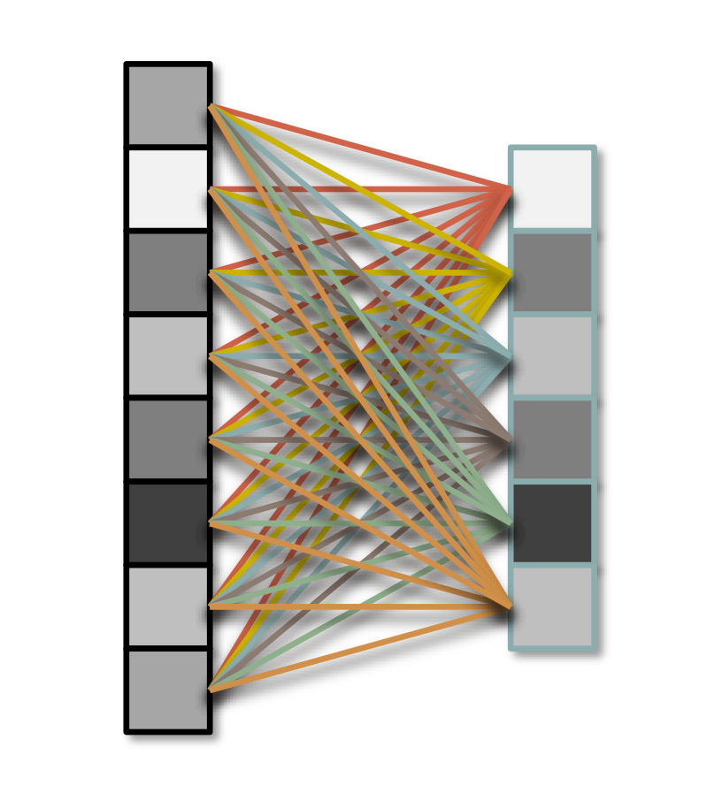
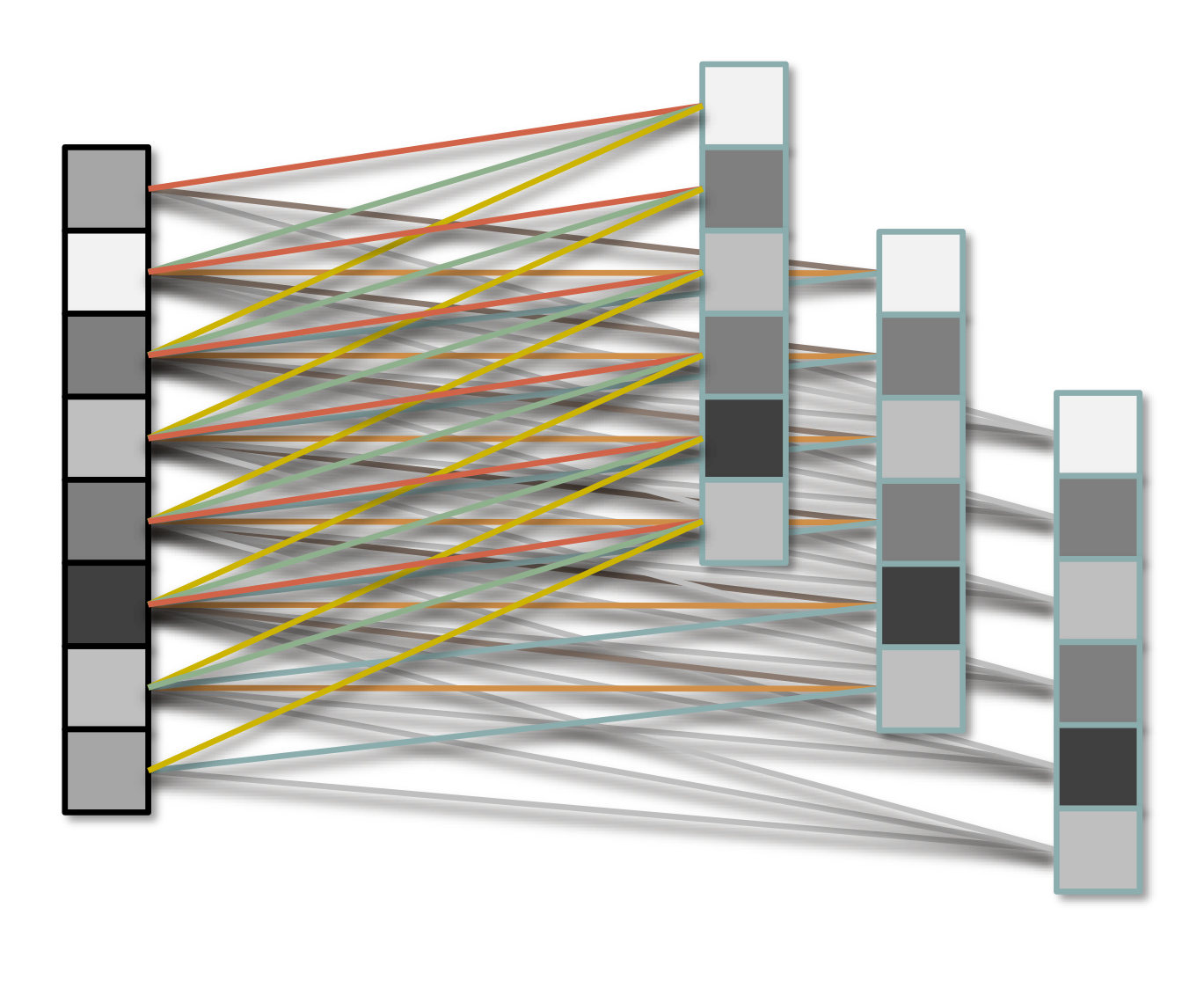
The simplest network architecture…
Each unit is connected to all units in previous layer.
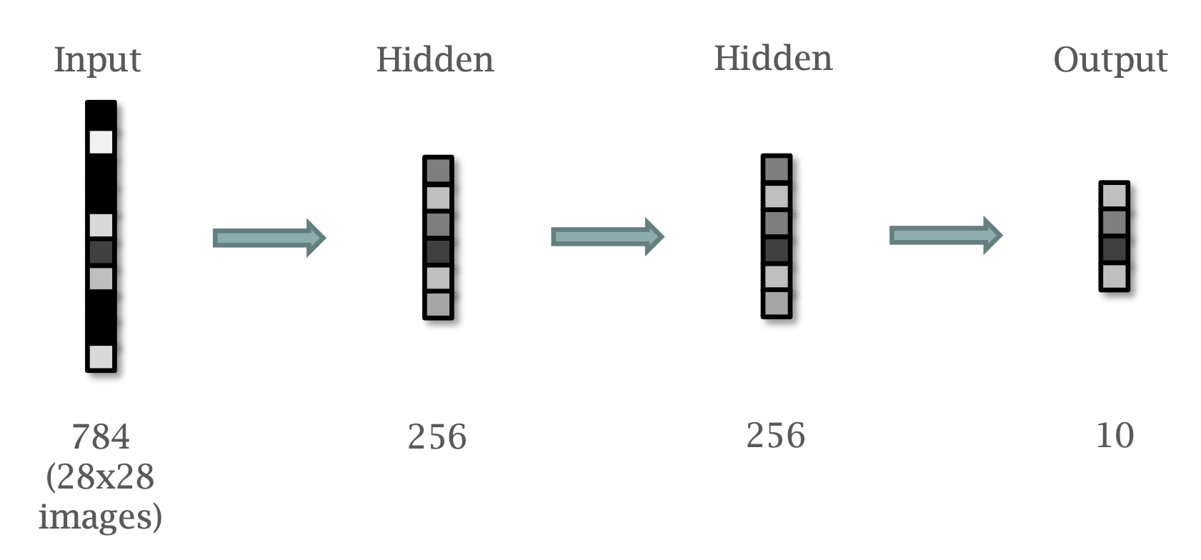
The “Hello World” of neural networks.
class Model(nn.Module):
    def __init__(self):
        super().__init__()
        self.input = nn.Linear(784, 256)
        self.hidden = nn.Linear(256, 256)
        self.output = nn.Linear(256, 10)

    def forward(self, x):
        x = x.view(x.shape[0], -1)
        x = F.relu(self.input(x))
        x = F.relu(self.hidden(x))
return self.output(x)class Model(nn.Module):
def __init__(self):
super().__init__()
self.input = nn.Linear(784, 256)
self.hidden = nn.Linear(256, 256)
self.output = nn.Linear(256, 10)
def forward(self, x):
x = x.view(x.shape[0], -1)
x = F.relu(self.input(x))
x = F.relu(self.hidden(x))
return self.output(x)class Model(nn.Module):
def __init__(self):
super().__init__()
self.input = nn.Linear(784, 256)
self.hidden = nn.Linear(256, 256)
self.output = nn.Linear(256, 10)
def forward(self, x):
x = x.view(x.shape[0], -1)
x = F.relu(self.input(x))
x = F.relu(self.hidden(x))
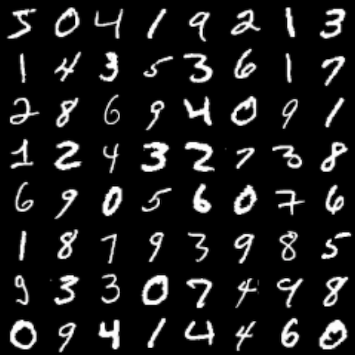
return self.output(x)MNIST is quite a special case.
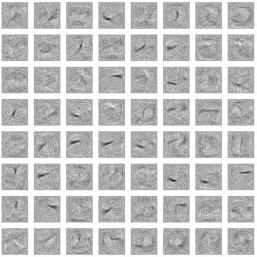
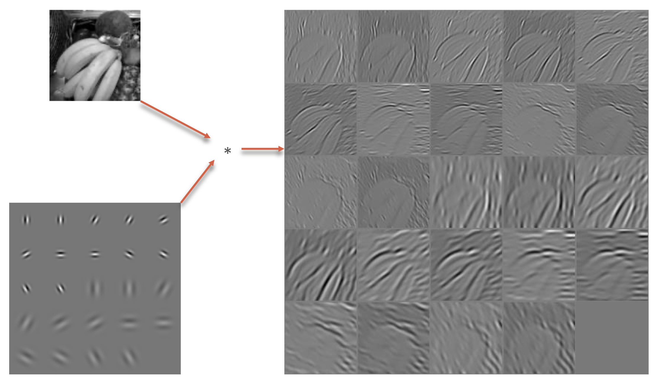
Note the stroke features detected by the various units.
Learned features lack translation invariance.
For more general imagery:
The computer vision revolution…
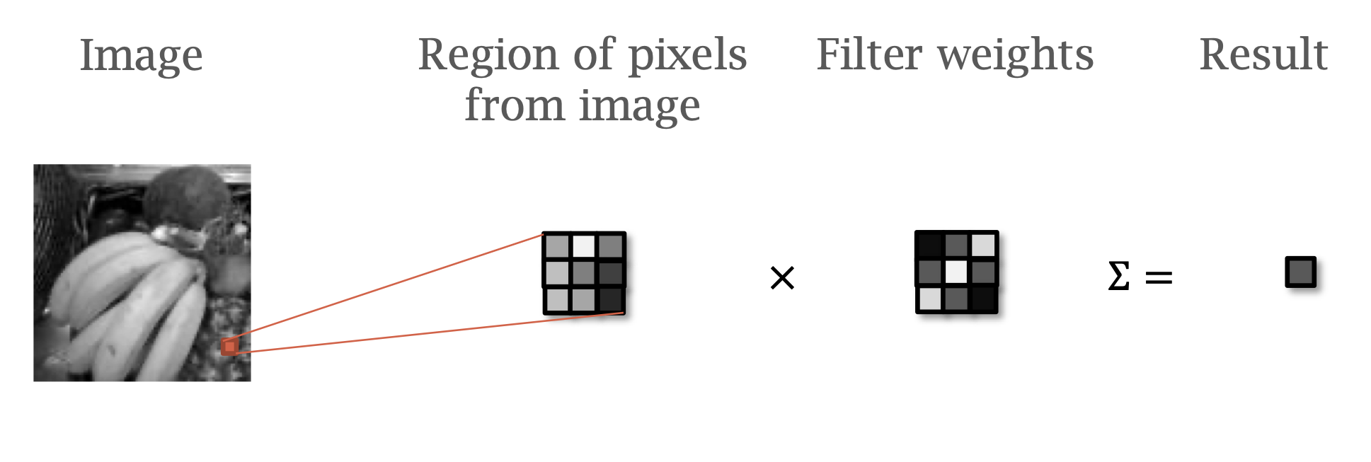
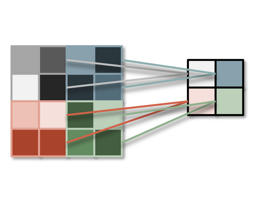
We have already discussed convolution.
Convolution detects features in a position independent manner.
Convolutional neural networks learn position independent filters.
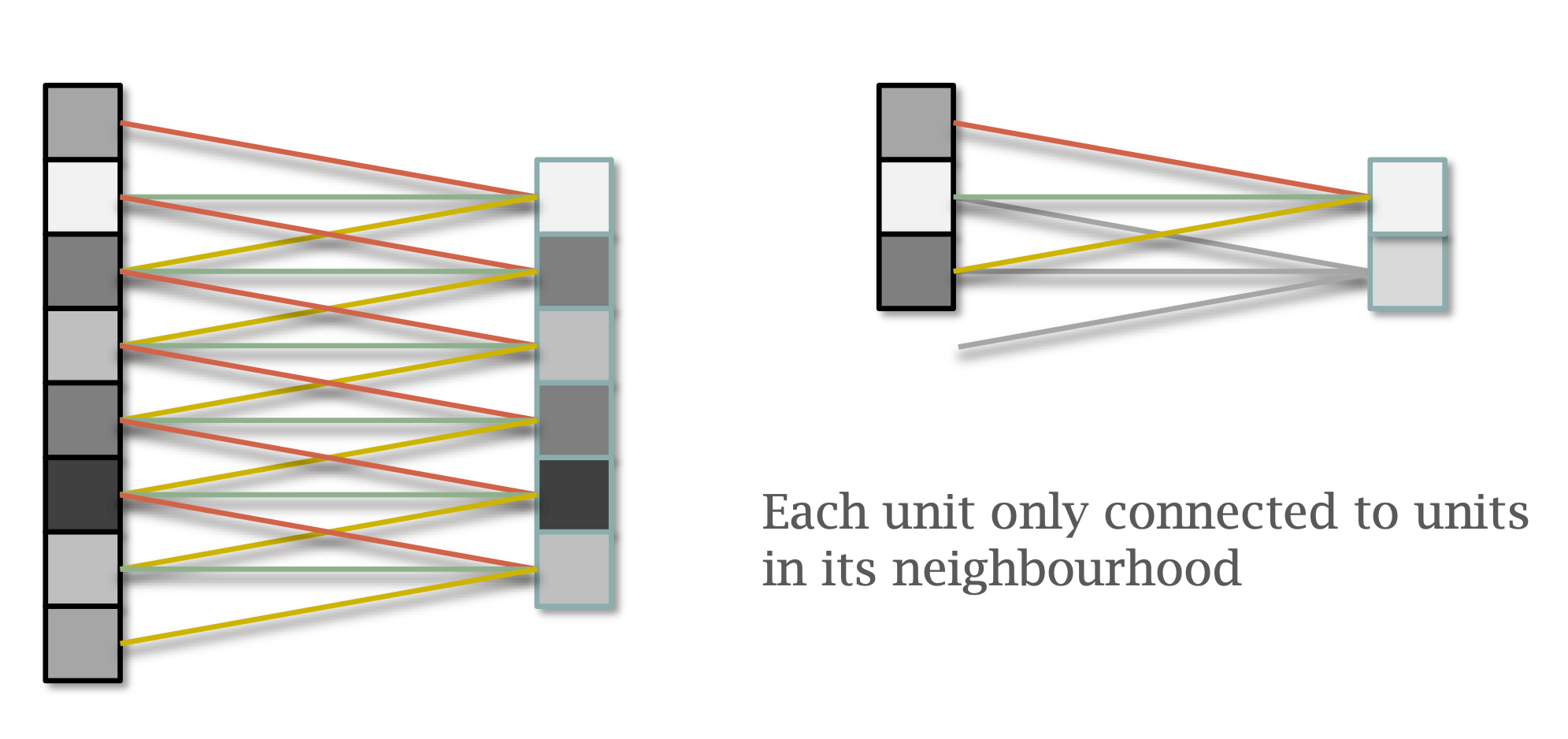
Each hidden unit is fully connected to all inputs.
Each hidden unit is only connected to inputs in its local neighbourhood.
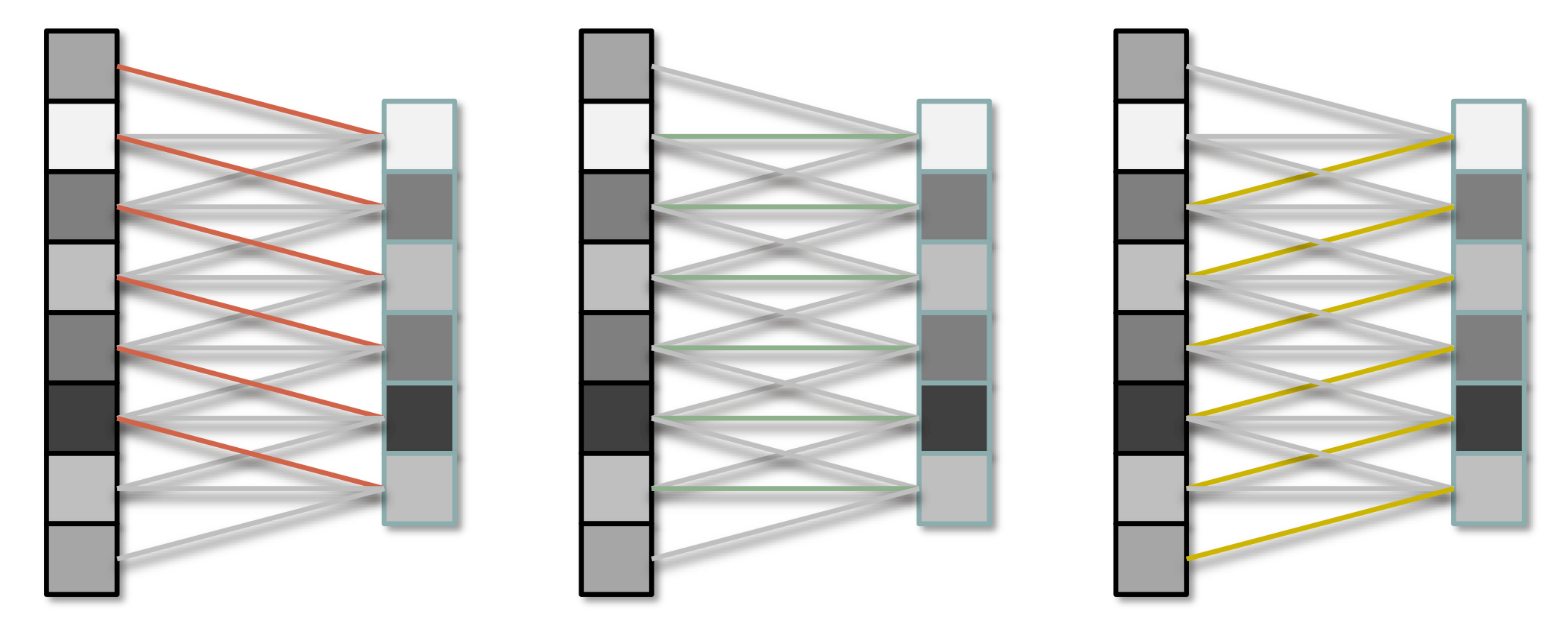
Each group of weights is shared between all units in the layer.
The values of the weights form a filter.
For practical computer vision, more than one filter must be used to extract a variety of features.
Multiple filter weights.
Output is image with multiple channels.
Convolution can be expressed as multiplication by weight matrix.
\[ y = f(Wx + b) \]
In subsequent layers, each filter connects to pixels in all channels in previous layer.
Take the maximum from each \((p \times p)\) pooling region.
Down sample the image by a factor of p.
We can also down-sample using strided convolution.
Visualisations are avalable at ConvNetJS by Andrej Karpathy.
https://cs.stanford.edu/people/karpathy/convnetjs/index.html
Source code for the site is available at: