BRIEF: Binary Robust Independent Elementary Features
ORB: Oriented FAST and rotated BRIEF
BRISK: Binary Robust Invariant Scalable Keypoints
FREAK: Fast REtinA Keypoint
… and many more
Descriptors
Describing a keypoint.
SIFT : Scale-Invariant Feature Transform
BRIEF : Binary Robust Independent Elementary Features
ORB : Oriented FAST and Rotated BRIEF
SIFT
Scale-Invariant Feature Transform
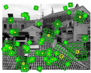
SIFT Features
Image content is transformed into features that are invariant to:
image translation
image rotation
image scale
SIFT Features
SIFT Features are partially invariant to:
illumination changes
affine transformations and 3D projections
SIFT Features
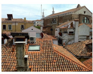
SIFT Features are suitable for detecting visual landmarks:
from different angles and distances.
with a different illumination.
DoG over Scale-Space Pyramid
Over different image pyramid levels:
Gaussian smoothing.
Difference-of-Gaussians (DoG) and find extrema.
Maxima suppression for edges.
SIFT Features
A SIFT feature is given by a vector computed at a local extreme point in the scale space.
\[ \langle p, s, r, f \rangle\]
SIFT Features
SIFT vector
SIFT Features
SIFT vector
SIFT Features
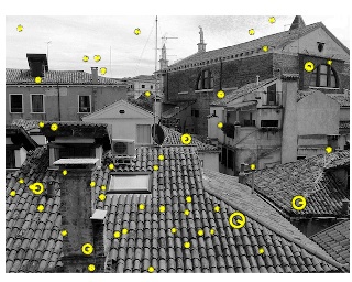
Input Image - Vedaldi & Fulkerson
From an input image we convert to grey scale then compute the Difference of Gaussians (DoG) and find the extrema.
SIFT Features
Keypoints, scale and orientation
We preserve the scale, and compute a peak of the histogram of orientations.
SIFT Features
locally rotated patch
We compute a local patch, based on the scale and orientation.
It is from this patch we compute the 128D feature descriptor vector.
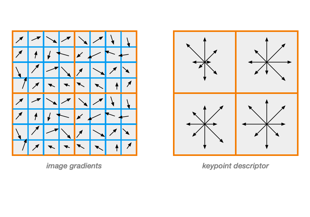
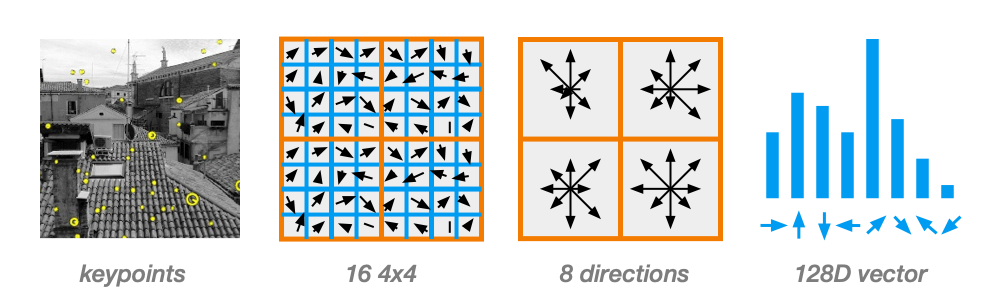
SIFT Descriptor
Compute image gradients in local 16x16 area at the selected scale.
Create an array of orientation histograms
8 orientations x 4x4 histogram array = 128 dimensions
SIFT Descriptor
sift descriptor
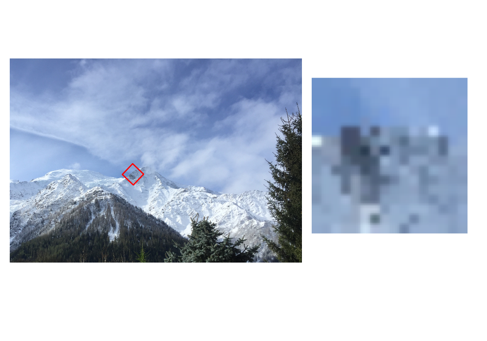
SIFT Descriptor
rotate and scale to 16x16
SIFT Descriptor
gradients and segregate to 16 x 4x4 regions
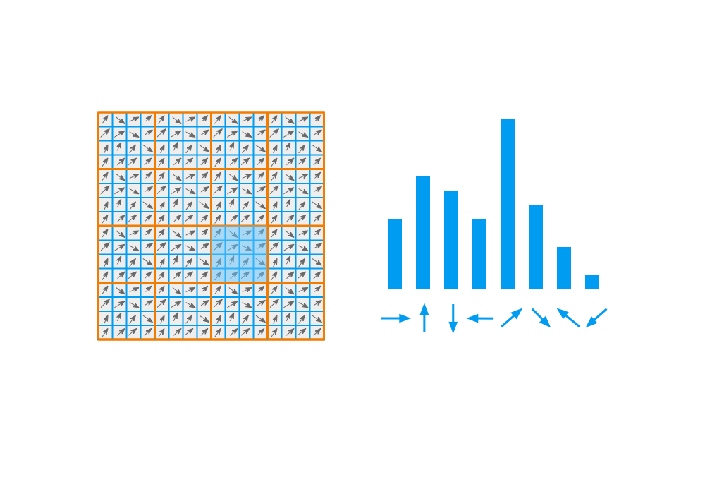
SIFT Descriptor
4x4 region to 8 direction bins
SIFT Descriptor
Concatenate all histograms to form a 128D vector.
concatenate histograms
SIFT Descriptor
Descriptor Summary
SIFT Features
Keypoints : Using DoG
Descriptor : Using Gradient Histogram
Dense SIFT
Variation of the SIFT feature, where the keypoints are sampled over a uniform grid in the image domain, rather than using the sparse points from the DoG.
Dense SIFT
At each uniform grid point:
Compute the SIFT descriptor.
Cluster the descriptors into a vocabulary.
K-means clustering.
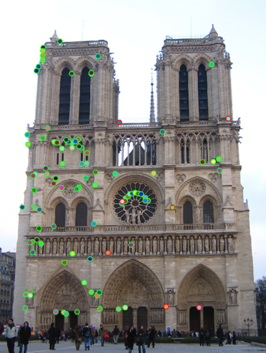
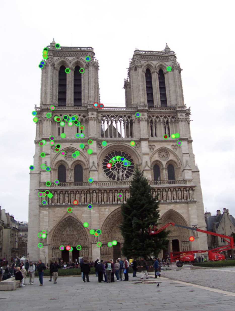
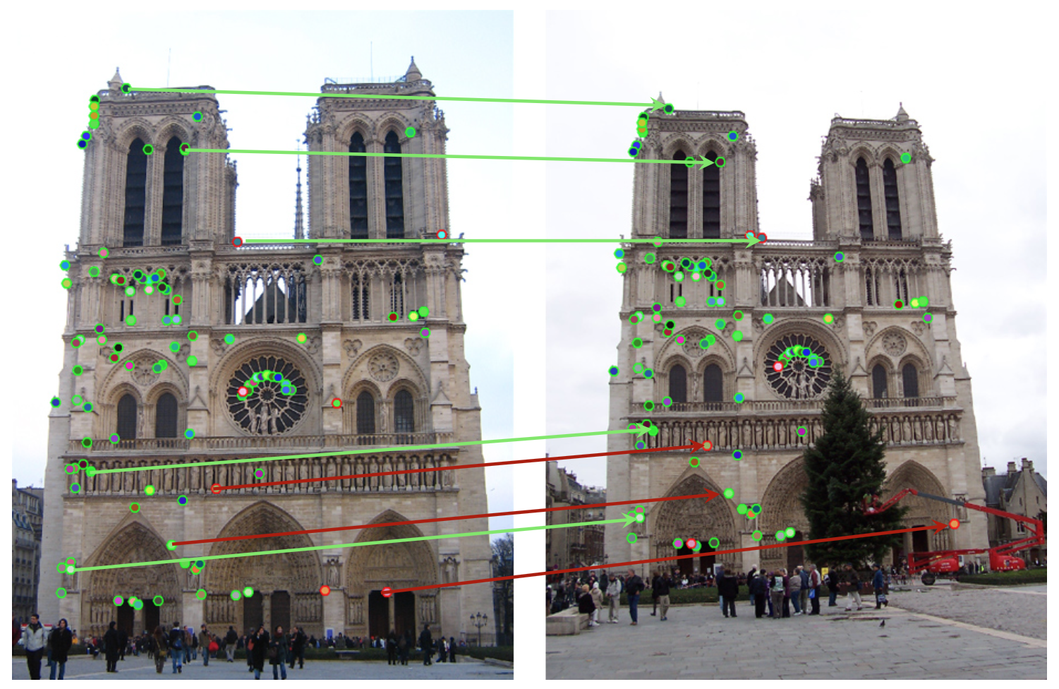
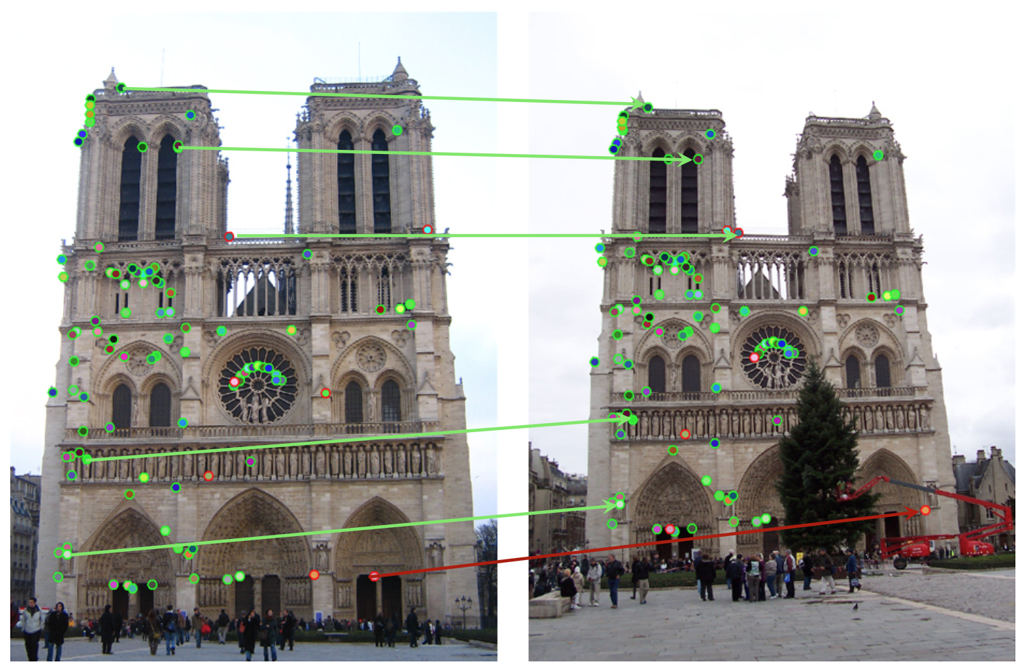
Matching
How do we match features from two images?
view 1
view 2
Distance Matching
descriptor distance
Ratio Test
Eliminate ambiguous matches for a query feature \(q\).
Find closest descriptors, \(p_1\) and \(p_2\) using Euclidian distance.
Test if distance to best match is smaller than a threshold:
\[d(q, p_1) < t\]
Accept only if the best match is substantially better than second:
\[\frac{d(q, p_1)}{d(q, p_2)} < \frac{1}{2}\]
Ratio Test
ratio test
Ratio Test
Lowe’s Ratio test works well.
There will still be a few outliers.
Outliers require extra treatment.
Binary Descriptors
Computing descriptors fast
Why Binary Descriptors?
Complex features such as SIFT work well, but…
SIFT is expensive to compute.
SIFT hashad patenting issues.
Binary descriptors are easy to compute and compare.