Visual Features - Keypoints
Computer Vision CMP-6035B
Dr. David Greenwood
Spring 2022
Contents
- Motivation
- Harris Corner Detection
- Shi-Tomasi Corner Detection
- Difference of Gaussian
Visual Features
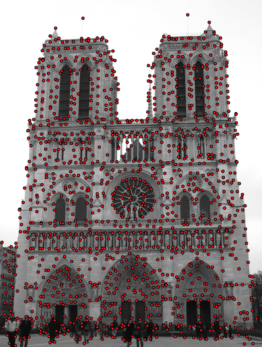
We want to find locally distinct features in an image.
- How do we find these features?
- How do we describe them?
Visual Features

We can take advantage of these locally distinct features for:
- image classification
- image retrieval
- correspondence between two images
- 3D reconstruction
Visual Features
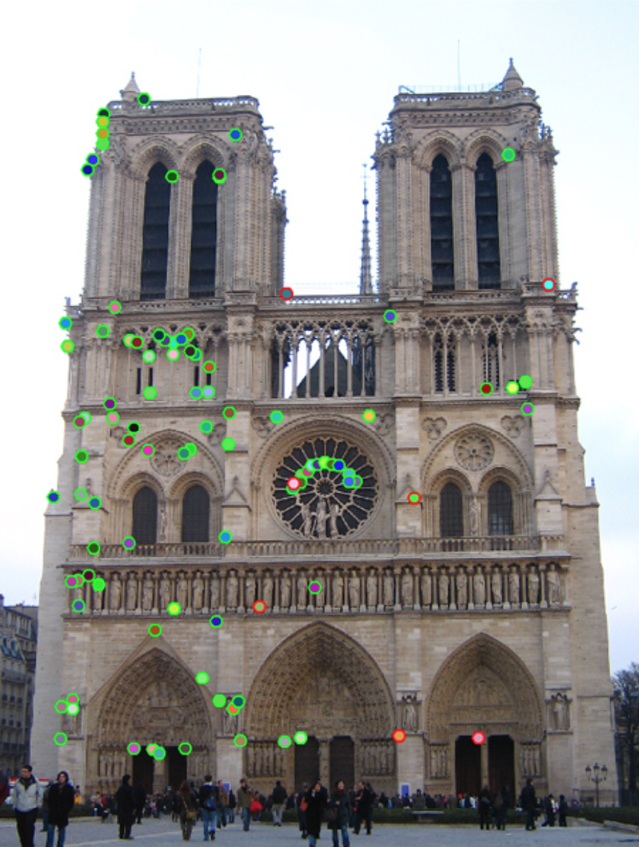
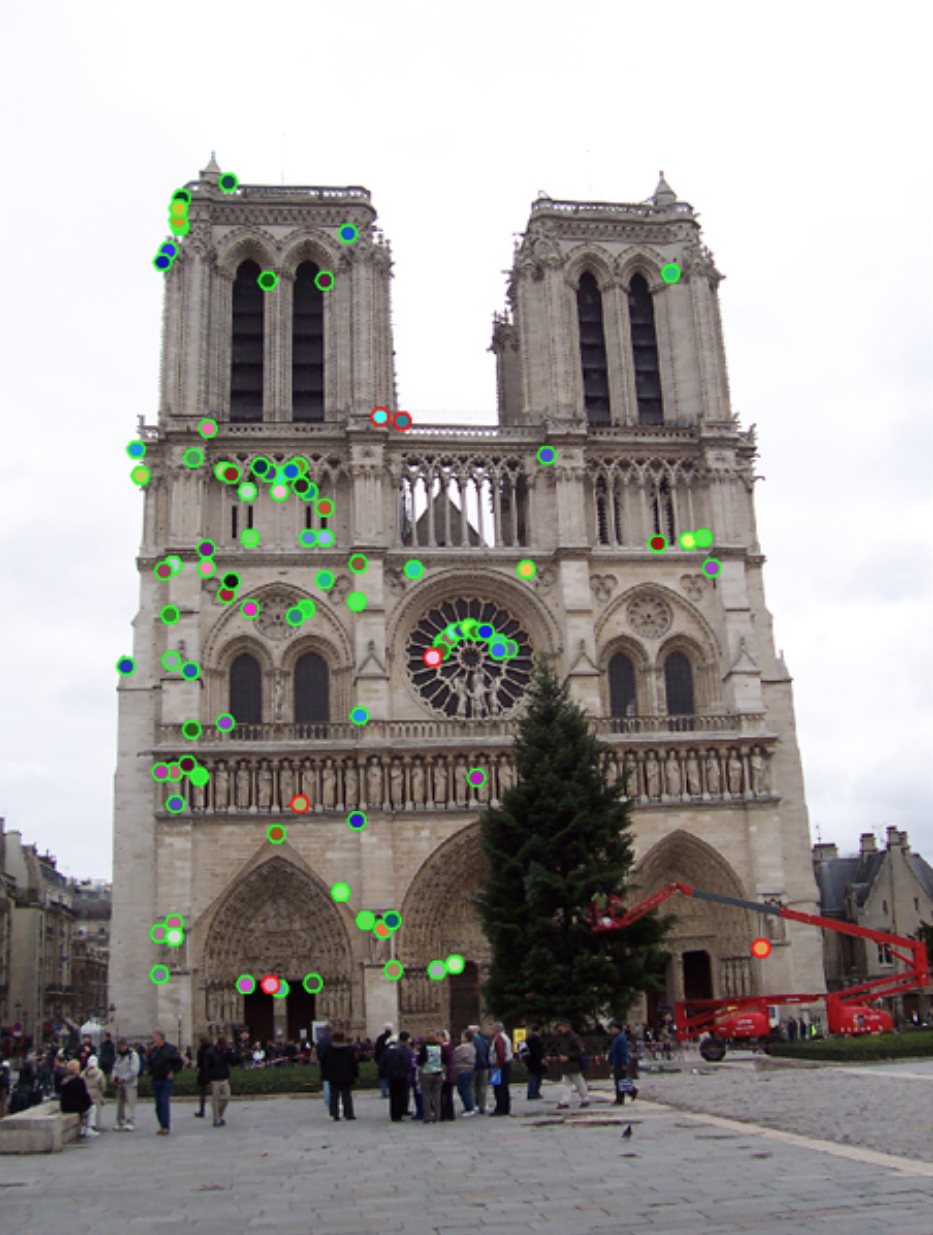
Keypoint and Descriptor
An important distinction:
- Keypoint is a distinct location in an image
- Descriptor is a summary description of that neighbourhood.
Keypoint and Descriptor

keypoint: \((x, ~y)\)
descriptor at the keypoint:
\[ \begin{bmatrix} 0.02 \\ 0.01 \\ 0.10 \\ 0.05 \\ 0.01 \\ ... \end{bmatrix} \]
Keypoints
Finding locally distinct points.
- Harris Corner Detection
- Shi-Tomasi Corner Detection
- Förstner operator
- Difference of Gaussians (DoG)
Corners
Corners are often highly distinct points.
Corners

Corners
- Corners are often highly distinct points.
- Edges are a rapid change in pixel value.
- Corners are formed from two orthogonal edges.
- Corners are invariant to translation, rotation and illumination.
Finding Corners
To find corners we need to search for intensity changes in two directions.
Finding Corners
Compute the SSD of pixels in the neighbourhood \(W\) around \((x, ~y)\).
\[ f(x, y) = \sum_{(u, v) \in W_{x,y} } (I(u, v) - I(u + \delta u , v + \delta v))^2 \]
Finding Corners
\[ f(x, y) = \sum_{(u, v) \in W_{x,y} } (I(u, v) - I(u + \delta u , v + \delta v))^2 \]
Using Taylor expansion, with Jacobian \(\left[J_x, J_y \right]\):
\[ I(u + \delta u , v + \delta v) \approx I(u, v) + \left[J_x, J_y \right] \begin{bmatrix} \delta u \\ \delta v \end{bmatrix} \]
Finding Corners
Taylor approximation leads to:
\[ f(x, y) = \sum_{(u, v) \in W_{x,y} } \left( [J_x, J_y] \begin{bmatrix} \delta u \\ \delta v \end{bmatrix}\right)^2 \]
Written in matrix form:
\[ f(x, y) = \sum_{(u, v) \in W_{x,y} } \begin{bmatrix} \delta u \\ \delta v \end{bmatrix}^T \begin{bmatrix} J_x^2 &J_xJ_y \\ J_xJ_y &J_y^2 \end{bmatrix} \begin{bmatrix} \delta u \\ \delta v \end{bmatrix} \]
Finding Corners
Given:
\[ f(x, y) = \sum_{(u, v) \in W_{x,y} } \begin{bmatrix} \delta u \\ \delta v \end{bmatrix}^T \begin{bmatrix} J_x^2 &J_xJ_y \\ J_xJ_y &J_y^2 \end{bmatrix} \begin{bmatrix} \delta u \\ \delta v \end{bmatrix} \]
Move the summation inside the matrix:
\[ f(x, y) = \begin{bmatrix} \delta u \\ \delta v \end{bmatrix}^T \begin{bmatrix} \sum_{W}J_x^2 &\sum_{W}J_xJ_y \\ \sum_{W}J_xJ_y &\sum_{W}J_y^2 \end{bmatrix} \begin{bmatrix} \delta u \\ \delta v \end{bmatrix} \]
Structure Matrix
\[ M = \begin{bmatrix} \sum_{W}J_x^2 &\sum_{W}J_xJ_y \\ \sum_{W}J_xJ_y &\sum_{W}J_y^2 \end{bmatrix} \]
Structure Matrix
- The structure matrix is key to finding edges and corners.
- Encodes the image intensity changes in a local area.
- built from image gradients.
\[ M = \begin{bmatrix} \sum_{W}J_x^2 &\sum_{W}J_xJ_y \\ \sum_{W}J_xJ_y &\sum_{W}J_y^2 \end{bmatrix} \]
Structure Matrix
Matrix built from image gradients.
\[ M = \begin{bmatrix} \sum_{W}J_x^2 &\sum_{W}J_xJ_y \\ \sum_{W}J_xJ_y &\sum_{W}J_y^2 \end{bmatrix} \]
Jacobians computed by convolution with gradient kernel, e.g. Sobel:
\[ \begin{aligned} J_x^2 &= (D_x * I)^2 \\ J_xJ_y &= (D_x * I) (D_y * I) \\ J_y^2 &= (D_y * I)^2 \end{aligned} \]
Structure Matrix
Matrix built from image gradients.
\[ M = \begin{bmatrix} \sum_{W}J_x^2 &\sum_{W}J_xJ_y \\ \sum_{W}J_xJ_y &\sum_{W}J_y^2 \end{bmatrix} \]
Jacobians using Sobel:
\[ D_x = \begin{bmatrix} 1 & 2 & 1 \\ 0 & 0 & 0 \\ \llap{-}1 & \llap{-}2 & \llap{-}1 \end{bmatrix}~, ~ D_y = \begin{bmatrix} 1 & 0 & \llap{-}1 \\ 2 & 0 & \llap{-}2 \\ 1 & 0 & \llap{-}1 \end{bmatrix} \]
Structure Matrix
Summarises the dominant gradient directions around a point.
\[ M = \begin{bmatrix} \sum_{W}J_x^2 &\sum_{W}J_xJ_y \\ \sum_{W}J_xJ_y &\sum_{W}J_y^2 \end{bmatrix} \]
Structure Matrix
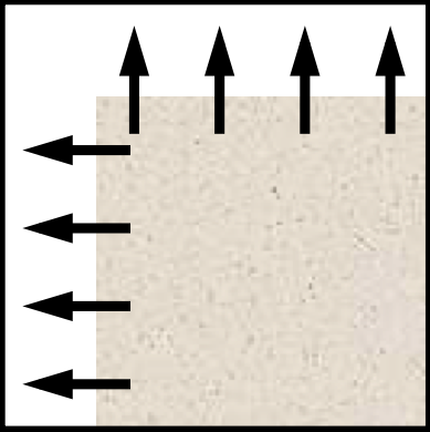
\[ M = \begin{bmatrix} \gg 1 &\approx 0 \\ \approx 0 &\gg 1 \end{bmatrix} \]
Structure Matrix
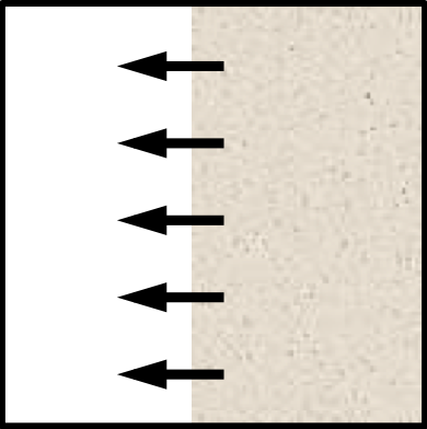
\[ M = \begin{bmatrix} \gg 1 &\approx 0 \\ \approx 0 &\approx 0 \end{bmatrix} \]
Structure Matrix
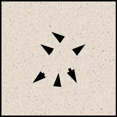
\[ M = \begin{bmatrix} \approx 0 &\approx 0 \\ \approx 0 &\approx 0 \end{bmatrix} \]
Corners from Structure Matrix
Consider points as corners if their structure matrix has two large Eigenvalues.

\[ M = \begin{bmatrix} \gg 1 &\approx 0 \\ \approx 0 &\gg 1 \end{bmatrix} \]
Corner Detection
Three similar approaches…
Harris, Shi-Tomasi and Förstner
Three similar approaches:
- 1987 Förstner
- 1988 Harris
- 1994 Shi-Tomasi
All rely on the structure matrix.
- Use different criteria for deciding if a point is a corner
- Förstner offers subpixel estimation
Harris Corner Criterion
Criterion:
\[ \begin{aligned} R &= det(M) - k(trace(M))^2 \\ &= \lambda_1 \lambda_2 - k(\lambda_1 + \lambda_2)^2 \end{aligned} \]
with \(k \in [0.04, 0.06]\):
\[ \begin{aligned} |R| &\approx 0 \Rightarrow \lambda_1 \approx \lambda_2 \approx 0 \\ R &< 0 \Rightarrow \lambda_1 \gg \lambda_2~ or ~\lambda_2 \gg \lambda_1 \\ R &\gg 0 \Rightarrow \lambda_1 \approx \lambda_2 \gg 0 \end{aligned} \]
Shi-Tomasi Criterion
Threshold smallest Eigenvalue:
\[ \lambda_{min}(M) = \frac{trace(M)}{2} - \frac{1}{2} \sqrt{trace(M)^2 - 4 det(M)} \]
corner:
\[ \lambda_{min}(M) \geq T \]
Förstner Criterion
- Similar to Harris corner detector.
- Criterion defined on the covariance matrix of possible shifts - inverse of \(M\).
- Similar criteria on error ellipse.
Non-Maxima Suppression
Within a local region, look for position with maximum value \(R\).
Which would be maximum here?
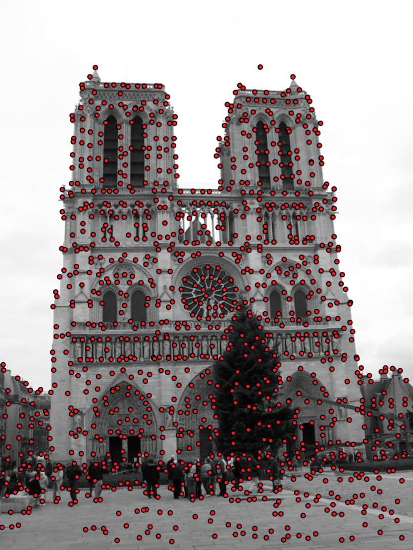
Harris Corner Example


Corner Detection in Practice
- RGB to grey scale conversion.
- Real images are noisy, so smoothing is recommended.
Corner Detection Algorithm
- Convolution with Sobel to obtain \(x, y\) derivatives.
- Multiplication of \(x, y\) derivatives to get \(J_xJ_x, J_yJ_y, J_xJ_y\).
- Summation of region, using box filter convolution.
- Apply criterion, e.g finding Eigenvalues.
Corner Detectors Compared
- All three detectors perform similarly.
- Förstner was first and also described subpixel estimation.
- Harris became the most popular corner detector.
- Shi-Tomasi seems to slightly outperform Harris.
- Many libraries use Shi-Tomasi as the default corner detector.
Difference of Gaussians
Difference of Gaussians (DoG)
Detecting edges, corners, and blobs…
DoG Keypoints
A variant of corner detection.
- Provides responses at corners, edges, and blobs.
- Blob = mainly constant region but different to its surroundings.
DoG over Scale Space Pyramid
Over different image pyramid levels
- Gaussian smoothing
- Difference-of-Gaussians: find extrema (over smoothing scales).
- maximal suppression at edges.
Difference of Gaussians
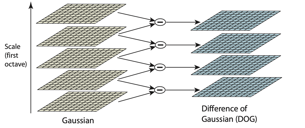
Difference of Gaussians
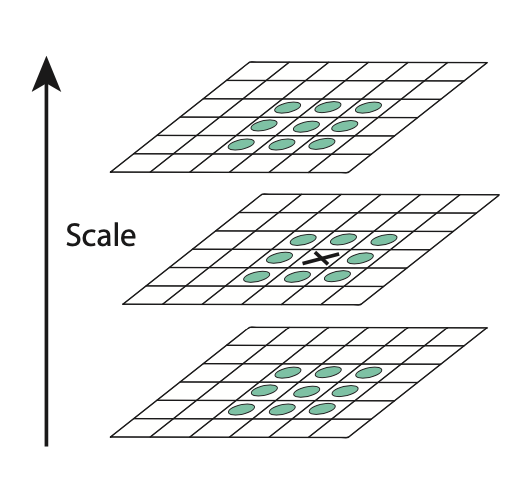
We search in \((x, y)\) and in the third dimension.
Difference of Gaussians
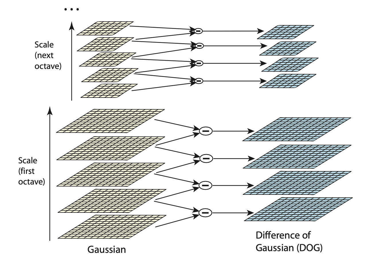
Difference of Gaussians
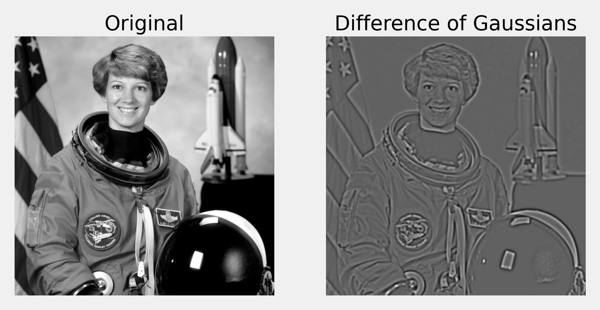
Difference of Gaussians
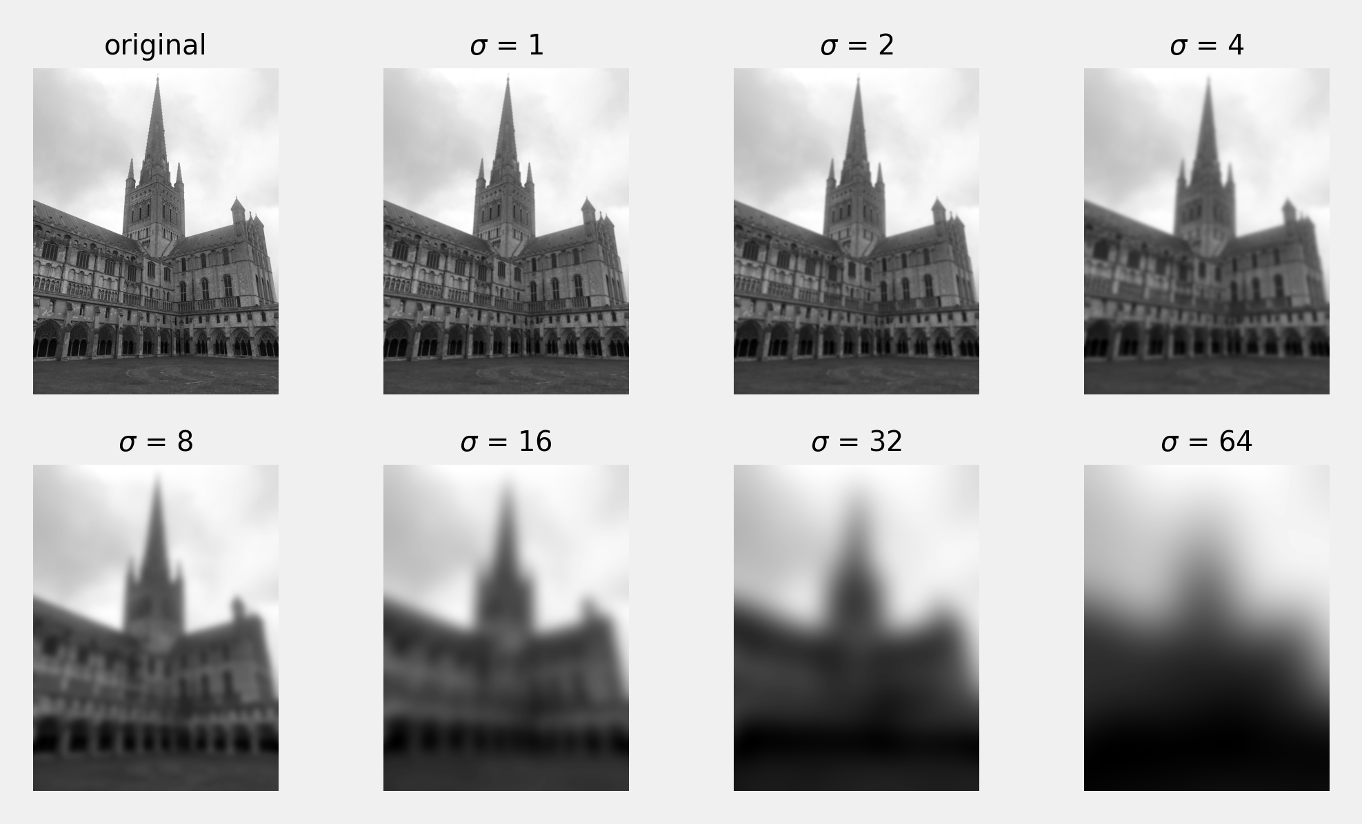
Difference of Gaussians
Blurring filters out high-frequencies (noise).
Subtracting differently blurred images from each other only keeps the frequencies that lie between the blur level of both images
DoG acts as a band-pass filter.
Difference of Gaussians
keypoints are the local extrema in the DoG over different scales.
Difference of Gaussians
The DoG finds blob-like and corner-like image structures but also has strong responses along edges.
- Edges are undesirable for matching.
- Eliminate edges via Eigenvalue test.
Summary
Two approaches for finding locally distinct points.
- Corners using the Structure Matrix.
- Difference of Gaussians
Reading:
- Forsyth, Ponce; Computer Vision: A modern approach, 2nd ed.
- A Combined Corner and Edge Detector, Harris, et al. 1988.
- Good Features to Track. Shi & Tomasi. 1994.